終于把機(jī)器學(xué)習(xí)中的混淆矩陣搞懂了！

作者：程序員小寒 2024-08-23 09:06:35

混淆矩陣是用于評估分類模型性能的表格。它通過將實(shí)際（真實(shí)）標(biāo)簽與預(yù)測標(biāo)簽進(jìn)行比較，提供分類問題的預(yù)測結(jié)果摘要。混淆矩陣本身是正方形（nxn），其中 n 是模型中的類別數(shù)。

大家好，我是小寒

今天給大家分享一個機(jī)器學(xué)習(xí)中一個重要的概念，混淆矩陣

混淆矩陣是用于評估分類模型性能的表格。它通過將實(shí)際（真實(shí)）標(biāo)簽與預(yù)測標(biāo)簽進(jìn)行比較，提供分類問題的預(yù)測結(jié)果摘要。

混淆矩陣本身是正方形（nxn），其中 n 是模型中的類別數(shù)。

對于二元分類問題，混淆矩陣由四個主要部分組成：

True Positive (TP, 真陽性)：實(shí)際為正類，預(yù)測也為正類的數(shù)量。
True Negative (TN, 真陰性)：實(shí)際為負(fù)類，預(yù)測也為負(fù)類的數(shù)量。
False Positive (FP, 假陽性)：實(shí)際為負(fù)類，預(yù)測卻為正類的數(shù)量，通常稱為"Type I 錯誤"或"誤報(bào)"。
False Negative (FN, 假陰性)：實(shí)際為正類，預(yù)測卻為負(fù)類的數(shù)量，通常稱為"Type II 錯誤"或"漏報(bào)"。

圖片

為什么要使用混淆矩陣？

混淆矩陣是評估分類模型性能的基本工具。

錯誤分析
它有助于識別模型所犯的錯誤類型，無論模型更容易出現(xiàn)假陽性還是假陰性，這在應(yīng)用范圍內(nèi)（例如在醫(yī)學(xué)診斷中）可能至關(guān)重要。
模型改進(jìn)
通過分析混淆矩陣，你可以專注于改進(jìn)模型的特定方面，例如減少誤報(bào)或提高召回率。
類別不平衡處理
在類別不平衡的情況下，一個類別出現(xiàn)的頻率高于另一個類別，單憑準(zhǔn)確率可能會產(chǎn)生誤導(dǎo)。
混淆矩陣可讓你更好地了解模型在每個類別中的表現(xiàn)。
性能指標(biāo)計(jì)算

分類中的評估指標(biāo)

1.準(zhǔn)確率

準(zhǔn)確率是分類任務(wù)中最簡單的評估指標(biāo)之一，用來衡量模型預(yù)測正確的比例。

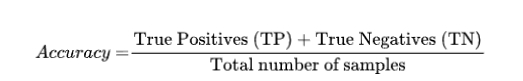
準(zhǔn)確率的局限性

當(dāng)處理不平衡的數(shù)據(jù)集時，一個類別的數(shù)量遠(yuǎn)遠(yuǎn)超過其他類別，準(zhǔn)確率可能會產(chǎn)生誤導(dǎo)。

例如，在 95％的樣本屬于同一類的數(shù)據(jù)集中，預(yù)測所有實(shí)例為多數(shù)類的模型的準(zhǔn)確率為 95％，但在識別少數(shù)類時則無效。

import matplotlib.pyplot as plt
import seaborn as sns
from sklearn.metrics import confusion_matrix, accuracy_score

# Example true labels (ytest) and predicted labels (ypred)
ytest = [0, 1, 0, 1, 0, 1, 0, 0, 1, 1]
ypred = [0, 1, 0, 0, 0, 1, 0, 1, 1, 1]

# Calculate confusion matrix
cm = confusion_matrix(ytest, ypred)

# Create a heatmap
plt.figure(figsize=(6, 4))
sns.heatmap(cm, annot=True, fmt='d', cmap='Blues', cbar=False,
            xticklabels=['1', '0'],
            yticklabels=['1', '0'])

# Add labels and title
plt.xlabel('Predicted Classes')
plt.ylabel('Actual Classes')
plt.title('Confusion Matrix')

# Calculate and display accuracy
accuracy = accuracy_score(ytest, ypred)
plt.text(2.3, 1.5, f'Accuracy: {accuracy:.2f}', fontsize=14, color='black', weight='bold')

plt.show()

圖片

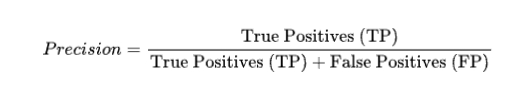
2.精度

精度用來衡量模型預(yù)測為正類的樣本中實(shí)際為正類的比例。

import matplotlib.pyplot as plt
import seaborn as sns
from sklearn.metrics import confusion_matrix, precision_score

# Example true labels (ytest) and predicted labels (ypred)
ytest = ['spam', 'spam', 'ham', 'spam', 'ham', 'spam', 'spam', 'ham', 'spam', 'spam', 'ham', 'spam', 'ham', 'ham', 'ham']
ypred = ['spam', 'spam', 'spam', 'spam', 'ham', 'spam', 'spam', 'ham', 'spam', 'spam', 'ham', 'ham', 'ham', 'ham', 'ham']

# Calculate the confusion matrix
cm = confusion_matrix(ytest, ypred, labels=['spam', 'ham'])
print("Confusion Matrix:\n", cm)

# Calculate precision
precision = precision_score(ytest, ypred, pos_label='spam')
print("Precision:", precision)

# Create a heatmap for the confusion matrix
plt.figure(figsize=(8, 6))
ax = sns.heatmap(cm, annot=True, fmt='d', cmap='viridis', cbar=False,
                 xticklabels=['Predicted Spam', 'Predicted Ham'],
                 yticklabels=['Actual Spam', 'Actual Ham'])

# Set labels and title
plt.xlabel('Predicted Classes')
plt.ylabel('Actual Classes')
plt.title(f'Confusion Matrix\nPrecision: {precision:.2f}')

# Show the plot
plt.show()

圖片

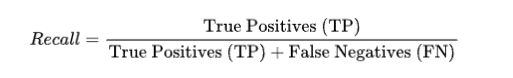
3.召回率

召回率用來衡量實(shí)際為正類的樣本中模型預(yù)測為正類的比例。

import matplotlib.pyplot as plt
import seaborn as sns
from sklearn.metrics import confusion_matrix, recall_score

# Example true labels (ytest) and predicted labels (ypred)
ytest = ['positive', 'positive', 'negative', 'positive', 'negative']
ypred = ['positive', 'negative', 'negative', 'positive', 'positive']

# Calculate the confusion matrix
cm = confusion_matrix(ytest, ypred, labels=['positive', 'negative'])


# Calculate recall
recall = recall_score(ytest, ypred, pos_label='positive')


# Create a heatmap for the confusion matrix
plt.figure(figsize=(6, 4))
ax = sns.heatmap(cm, annot=True, fmt='d', cmap='viridis', cbar=False,
                 xticklabels=['Predicted Positive', 'Predicted Negative'],
                 yticklabels=['Actual Positive', 'Actual Negative'])

# Set labels and title
plt.xlabel('Predicted Classes')
plt.ylabel('Actual Classes')
plt.title(f'Confusion Matrix\nRecall: {recall:.2f}')

# Show the plot
plt.show()

圖片