NLP 與 Python:構建知識圖譜實戰案例

概括
積累了一兩周,好久沒做筆記了,今天,我將展示在之前兩周的實戰經驗:如何使用 Python 和自然語言處理構建知識圖譜。
網絡圖是一種數學結構,用于表示點之間的關系,可通過無向/有向圖結構進行可視化展示。它是一種將相關節點映射的數據庫形式。
知識庫是來自不同來源信息的集中存儲庫,如維基百科、百度百科等。
知識圖譜是一種采用圖形數據模型的知識庫。簡單來說,它是一種特殊類型的網絡圖,用于展示現實世界實體、事實、概念和事件之間的關系。2012年,谷歌首次使用“知識圖譜”這個術語,用于介紹他們的模型。

目前,大多數公司都在建立數據湖,這是一個中央數據庫,它可以收集來自不同來源的各種類型的原始數據(包括結構化和非結構化數據)。因此,人們需要工具來理解所有這些不同信息的意義。知識圖譜越來越受歡迎,因為它可以簡化大型數據集的探索和發現。簡單來說,知識圖譜將數據和相關元數據連接起來,因此可以用來構建組織信息資產的全面表示。例如,知識圖譜可以替代您需要查閱的所有文件,以查找特定的信息。
知識圖譜被視為自然語言處理領域的一部分,因為要構建“知識”,需要進行“語義增強”過程。由于沒有人想要手動執行此任務,因此我們需要使用機器和自然語言處理算法來完成此任務。
我將解析維基百科并提取一個頁面,用作本教程的數據集(下面的鏈接)。
俄烏戰爭 - 維基百科 俄烏戰爭是俄羅斯與俄羅斯支持的分離主義者之間持續的國際沖突,以及...... en.wikipedia.org
特別是將通過:
- 設置:使用維基百科API進行網頁爬取以讀取包和數據。
- NLP使用SpaCy:對文本進行分句、詞性標注、依存句法分析和命名實體識別。
- 提取實體及其關系:使用Textacy庫來識別實體并建立它們之間的關系。
- 網絡圖構建:使用NetworkX庫來創建和操作圖形結構。
- 時間軸圖:使用DateParser庫來解析日期信息并生成時間軸圖。
設置
首先導入以下庫:
## for data
import pandas as pd  #1.1.5
import numpy as np  #1.21.0

## for plotting
import matplotlib.pyplot as plt  #3.3.2

## for text
import wikipediaapi  #0.5.8
import nltk  #3.8.1
import re

## for nlp
import spacy  #3.5.0
from spacy import displacy
import textacy  #0.12.0

## for graph
import networkx as nx  #3.0 (also pygraphviz==1.10)

## for timeline
import dateparser #1.1.7
Wikipedia-api是一個Python庫,可輕松解析Wikipedia頁面。我們將使用這個庫來提取所需的頁面,但會排除頁面底部的所有“注釋”和“參考文獻”內容。

簡單地寫出頁面的名稱:
topic = "Russo-Ukrainian War"

wiki = wikipediaapi.Wikipedia('en')
page = wiki.page(topic)
txt = page.text[:page.text.find("See also")]
txt[0:500] + " ..."
通過從文本中識別和提取subjects-actions-objects來繪制歷史事件的關系圖譜(因此動詞是關系)。
自然語言處理
要構建知識圖譜,首先需要識別實體及其關系。因此,需要使用自然語言處理技術處理文本數據集。
目前,最常用于此類任務的庫是SpaCy,它是一種開源軟件,用于高級自然語言處理,利用Cython(C+Python)進行加速。SpaCy使用預訓練的語言模型對文本進行標記化,并將其轉換為“文檔”對象,該對象包含模型預測的所有注釋。
#python -m spacy download en_core_web_sm

nlp = spacy.load("en_core_web_sm")
doc = nlp(txt)
NLP模型的第一個輸出是句子分割(中文有自己的分詞規則):即確定句子的起始和結束位置的問題。通常,它是通過基于標點符號對段落進行分割來完成的。現在我們來看看SpaCy將文本分成了多少個句子:
# from text to a list of sentences
lst_docs = [sent for sent in doc.sents]
print("tot sentences:", len(lst_docs))
現在,對于每個句子,我們將提取實體及其關系。為了做到這一點,首先需要了解詞性標注(POS):即用適當的語法標簽標記句子中的每個單詞的過程。以下是可能標記的完整列表(截至今日):
- ADJ: 形容詞,例如big,old,green,incomprehensible,first
- ADP: 介詞,例如in,to,during
- ADV: 副詞,例如very,tomorrow,down,where,there
- AUX: 助動詞,例如is,has(done),will(do),should(do)
- CONJ: 連詞,例如and,or,but
- CCONJ: 并列連詞,例如and,or,but
- DET: 限定詞,例如a,an,the
- INTJ: 感嘆詞,例如psst,ouch,bravo,hello
- NOUN: 名詞,例如girl,cat,tree,air,beauty
- NUM: 數詞,例如1,2017,one,seventy-seven,IV,MMXIV
- PART: 助詞,例如's,not
- PRON: 代詞,例如I,you,he,she,myself,themselves,somebody
- PROPN: 專有名詞,例如Mary,John,London,NATO,HBO
- PUNCT: 標點符號,例如.,(,),?
- SCONJ: 從屬連詞,例如if,while,that
- SYM: 符號,例如$,%,§,?,+,-,×,÷,=,:),表情符號
- VERB: 動詞,例如run,runs,running,eat,ate,eating
- X: 其他,例如sfpksdpsxmsa
- SPACE: 空格,例如
僅有詞性標注是不夠的,模型還會嘗試理解單詞對之間的關系。這個任務稱為依存句法分析(Dependency Parsing,DEP)。以下是可能的標簽完整列表(截至今日)。
- ACL:作為名詞從句的修飾語
- ACOMP:形容詞補語
- ADVCL:狀語從句修飾語
- ADVMOD:狀語修飾語
- AGENT:主語中的動作執行者
- AMOD:形容詞修飾語
- APPOS:同位語
- ATTR:主謂結構中的謂語部分
- AUX:助動詞
- AUXPASS:被動語態中的助動詞
- CASE:格標記
- CC:并列連詞
- CCOMP:從句補足語
- COMPOUND:復合修飾語
- CONJ:連接詞
- CSUBJ:主語從句
- CSUBJPASS:被動語態中的主語從句
- DATIVE:與雙賓語動詞相關的間接賓語
- DEP:未分類的依賴
- DET:限定詞
- DOBJ:直接賓語
- EXPL:人稱代詞
- INTJ:感嘆詞
- MARK:標記
- META:元素修飾語
- NEG:否定修飾語
- NOUNMOD:名詞修飾語
- NPMOD:名詞短語修飾語
- NSUBJ:名詞從句主語
- NSUBJPASS:被動語態中的名詞從句主語
- NUMMOD:數字修飾語
- OPRD:賓語補足語
- PARATAXIS:并列結構
- PCOMP:介詞的補足語
- POBJ:介詞賓語
- POSS:所有格修飾語
- PRECONJ:前置連詞
- PREDET:前置限定詞
- PREP:介詞修飾語
- PRT:小品詞
- PUNCT:標點符號
- QUANTMOD:量詞修飾語
- RELCL:關系從句修飾語
- ROOT:句子主干
- XCOMP:開放性從句補足語
舉個例子來理解POS標記和DEP解析:
# take a sentence
i = 3
lst_docs[i]
檢查 NLP 模型預測的 POS 和 DEP 標簽:
for token in lst_docs[i]:
    print(token.text, "-->", "pos: "+token.pos_, "|", "dep: "+token.dep_, "")
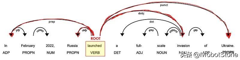
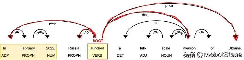
SpaCy提供了一個圖形工具來可視化這些注釋:
from spacy import displacy

displacy.render(lst_docs[i], style="dep", options={"distance":100})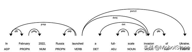
最重要的標記是動詞 ( POS=VERB ),因為它是句子中含義的詞根 ( DEP=ROOT )。
助詞,如副詞和副詞 ( POS=ADV/ADP ),通常作為修飾語 ( *DEP=mod ) 與動詞相關聯,因為它們可以修飾動詞的含義。例如,“ travel to ”和“ travel from ”具有不同的含義,即使詞根相同(“ travel ”)。
在與動詞相連的單詞中,必須有一些名詞(POS=PROPN/NOUN)作為句子的主語和賓語( *DEP=nsubj/obj )。

名詞通常位于形容詞 ( POS=ADJ ) 附近,作為其含義的修飾語 ( DEP=amod )。例如,在“好人”和“壞人”中,形容詞賦予名詞“人”相反的含義。
SpaCy執行的另一個很酷的任務是命名實體識別(NER)。命名實體是“真實世界中的對象”(例如人、國家、產品、日期),模型可以在文檔中識別各種類型的命名實體。以下是可能的所有標簽的完整列表(截至今日):
- 人名: 包括虛構人物。
- 國家、宗教或政治團體:民族、宗教或政治團體。
- 地點:建筑、機場、高速公路、橋梁等。
- 公司、機構等:公司、機構等。
- 地理位置:國家、城市、州。
- 地點:非國家地理位置,山脈、水域等。
- 產品:物體、車輛、食品等(不包括服務)。
- 事件:命名颶風、戰斗、戰爭、體育賽事等。
- 藝術作品:書籍、歌曲等的標題。
- 法律:成為法律的指定文件。
- 語言:任何命名的語言。
- 日期:絕對或相對日期或期間。
- 時間:小于一天的時間。
- 百分比:百分比,包括“%”。
- 貨幣:貨幣價值,包括單位。
- 數量:衡量重量或距離等。
- 序數: “第一”,“第二”等。
- 基數:不屬于其他類型的數字。
for tag in lst_docs[i].ents:
    print(tag.text, f"({tag.label_})")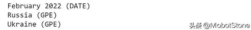
或者使用SpaCy圖形工具更好:
displacy.render(lst_docs[i], style="ent")
這對于我們想要向知識圖譜添加多個屬性的情況非常有用。
接下來,使用NLP模型預測的標簽,我們可以提取實體及其關系。
實體和關系抽取
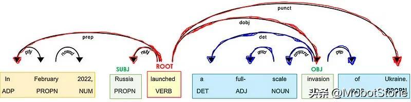
這個想法很簡單,但實現起來可能會有些棘手。對于每個句子,我們將提取主語和賓語以及它們的修飾語、復合詞和它們之間的標點符號。
可以通過兩種方式完成:
- 手動方式:可以從基準代碼開始,該代碼可能必須稍作修改并針對您特定的數據集/用例進行調整。
def extract_entities(doc):
    a, b, prev_dep, prev_txt, prefix, modifier = "", "", "", "", "", ""
    for token in doc:
        if token.dep_ != "punct":
            ## prexif --> prev_compound + compound
            if token.dep_ == "compound":
                prefix = prev_txt +" "+ token.text if prev_dep == "compound" else token.text

            ## modifier --> prev_compound + %mod
            if token.dep_.endswith("mod") == True:
                modifier = prev_txt +" "+ token.text if prev_dep == "compound" else token.text

            ## subject --> modifier + prefix + %subj
            if token.dep_.find("subj") == True:
                a = modifier +" "+ prefix + " "+ token.text
                prefix, modifier, prev_dep, prev_txt = "", "", "", ""

            ## if object --> modifier + prefix + %obj
            if token.dep_.find("obj") == True:
                b = modifier +" "+ prefix +" "+ token.text

            prev_dep, prev_txt = token.dep_, token.text

    # clean
    a = " ".join([i for i in a.split()])
    b = " ".join([i for i in b.split()])
    return (a.strip(), b.strip())


# The relation extraction requires the rule-based matching tool,
# an improved version of regular expressions on raw text.
def extract_relation(doc, nlp):
    matcher = spacy.matcher.Matcher(nlp.vocab)
    p1 = [{'DEP':'ROOT'},
          {'DEP':'prep', 'OP':"?"},
          {'DEP':'agent', 'OP':"?"},
          {'POS':'ADJ', 'OP':"?"}]
    matcher.add(key="matching_1", patterns=[p1])
    matches = matcher(doc)
    k = len(matches) - 1
    span = doc[matches[k][1]:matches[k][2]]
    return span.text
讓我們在這個數據集上試試看,看看通常的例子:
## extract entities
lst_entities = [extract_entities(i) for i in lst_docs]

## example
lst_entities[i]
## extract relations
lst_relations = [extract_relation(i,nlp) for i in lst_docs]

## example
lst_relations[i]
## extract attributes (NER)
lst_attr = []
for x in lst_docs:
    attr = ""
    for tag in x.ents:
        attr = attr+tag.text if tag.label_=="DATE" else attr+""
    lst_attr.append(attr)

## example
lst_attr[i]
第二種方法是使用Textacy,這是一個基于SpaCy構建的庫,用于擴展其核心功能。這種方法更加用戶友好,通常也更準確。
## extract entities and relations
dic = {"id":[], "text":[], "entity":[], "relation":[], "object":[]}

for n,sentence in enumerate(lst_docs):
    lst_generators = list(textacy.extract.subject_verb_object_triples(sentence))
    for sent in lst_generators:
        subj = "_".join(map(str, sent.subject))
        obj  = "_".join(map(str, sent.object))
        relation = "_".join(map(str, sent.verb))
        dic["id"].append(n)
        dic["text"].append(sentence.text)
        dic["entity"].append(subj)
        dic["object"].append(obj)
        dic["relation"].append(relation)


## create dataframe
dtf = pd.DataFrame(dic)

## example
dtf[dtf["id"]==i]
讓我們也使用 NER 標簽(即日期)提取屬性:
## extract attributes
attribute = "DATE"
dic = {"id":[], "text":[], attribute:[]}

for n,sentence in enumerate(lst_docs):
    lst = list(textacy.extract.entities(sentence, include_types={attribute}))
    if len(lst) > 0:
        for attr in lst:
            dic["id"].append(n)
            dic["text"].append(sentence.text)
            dic[attribute].append(str(attr))
    else:
        dic["id"].append(n)
        dic["text"].append(sentence.text)
        dic[attribute].append(np.nan)

dtf_att = pd.DataFrame(dic)
dtf_att = dtf_att[~dtf_att[attribute].isna()]

## example
dtf_att[dtf_att["id"]==i]
已經提取了“知識”,接下來可以構建圖表了。
網絡圖
Python標準庫中用于創建和操作圖網絡的是NetworkX。我們可以從整個數據集開始創建圖形,但如果節點太多,可視化將變得混亂:
## create full graph
G = nx.from_pandas_edgelist(dtf, source="entity", target="object",
                            edge_attr="relation",
                            create_using=nx.DiGraph())


## plot
plt.figure(figsize=(15,10))

pos = nx.spring_layout(G, k=1)
node_color = "skyblue"
edge_color = "black"

nx.draw(G, pos=pos, with_labels=True, node_color=node_color,
        edge_color=edge_color, cmap=plt.cm.Dark2,
        node_size=2000, connectionstyle='arc3,rad=0.1')

nx.draw_networkx_edge_labels(G, pos=pos, label_pos=0.5,
                         edge_labels=nx.get_edge_attributes(G,'relation'),
                         font_size=12, font_color='black', alpha=0.6)
plt.show()
知識圖譜可以讓我們從大局的角度看到所有事物的相關性,但是如果直接看整張圖就沒有什么用處。因此,最好根據我們所需的信息應用一些過濾器。對于這個例子,我將只選擇涉及最常見實體的部分(基本上是最連接的節點):
dtf["entity"].value_counts().head()
## filter
f = "Russia"
tmp = dtf[(dtf["entity"]==f) | (dtf["object"]==f)]


## create small graph
G = nx.from_pandas_edgelist(tmp, source="entity", target="object",
                            edge_attr="relation",
                            create_using=nx.DiGraph())


## plot
plt.figure(figsize=(15,10))

pos = nx.nx_agraph.graphviz_layout(G, prog="neato")
node_color = ["red" if node==f else "skyblue" for node in G.nodes]
edge_color = ["red" if edge[0]==f else "black" for edge in G.edges]

nx.draw(G, pos=pos, with_labels=True, node_color=node_color,
        edge_color=edge_color, cmap=plt.cm.Dark2,
        node_size=2000, node_shape="o", connectionstyle='arc3,rad=0.1')

nx.draw_networkx_edge_labels(G, pos=pos, label_pos=0.5,
                        edge_labels=nx.get_edge_attributes(G,'relation'),
                        font_size=12, font_color='black', alpha=0.6)
plt.show()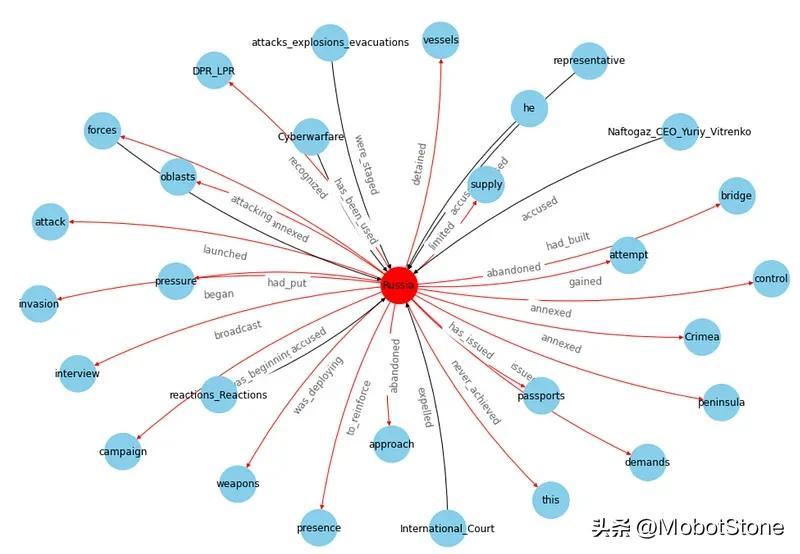
上面的效果已經不錯了。如果想讓它成為 3D 的話,可以使用以下代碼:
from mpl_toolkits.mplot3d import Axes3D

fig = plt.figure(figsize=(15,10))
ax = fig.add_subplot(111, projection="3d")
pos = nx.spring_layout(G, k=2.5, dim=3)

nodes = np.array([pos[v] for v in sorted(G) if v!=f])
center_node = np.array([pos[v] for v in sorted(G) if v==f])

edges = np.array([(pos[u],pos[v]) for u,v in G.edges() if v!=f])
center_edges = np.array([(pos[u],pos[v]) for u,v in G.edges() if v==f])

ax.scatter(*nodes.T, s=200, ec="w", c="skyblue", alpha=0.5)
ax.scatter(*center_node.T, s=200, c="red", alpha=0.5)

for link in edges:
    ax.plot(*link.T, color="grey", lw=0.5)
for link in center_edges:
    ax.plot(*link.T, color="red", lw=0.5)

for v in sorted(G):
    ax.text(*pos[v].T, s=v)
for u,v in G.edges():
    attr = nx.get_edge_attributes(G, "relation")[(u,v)]
    ax.text(*((pos[u]+pos[v])/2).T, s=attr)

ax.set(xlabel=None, ylabel=None, zlabel=None,
       xticklabels=[], yticklabels=[], zticklabels=[])
ax.grid(False)
for dim in (ax.xaxis, ax.yaxis, ax.zaxis):
    dim.set_ticks([])
plt.show()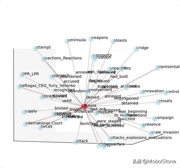
需要注意一點,圖形網絡可能很有用且漂亮,但它不是本教程的重點。知識圖譜最重要的部分是“知識”(文本處理),然后可以在數據幀、圖形或其他圖表上顯示結果。例如,我可以使用NER識別的日期來構建時間軸圖。
時間軸圖
首先,需要將被識別為“日期”的字符串轉換為日期時間格式。DateParser庫可以解析幾乎在網頁上常見的任何字符串格式中的日期。
def utils_parsetime(txt):
    x = re.match(r'.*([1-3][0-9]{3})', txt) #<--check if there is a year
    if x is not None:
        try:
            dt = dateparser.parse(txt)
        except:
            dt = np.nan
    else:
        dt = np.nan
    return dt
將它應用于屬性的數據框:
dtf_att["dt"] = dtf_att["date"].apply(lambda x: utils_parsetime(x))

## example
dtf_att[dtf_att["id"]==i]
將把它與實體關系的主要數據框結合起來:
tmp = dtf.copy()
tmp["y"] = tmp["entity"]+" "+tmp["relation"]+" "+tmp["object"]

dtf_att = dtf_att.merge(tmp[["id","y"]], how="left", on="id")
dtf_att = dtf_att[~dtf_att["y"].isna()].sort_values("dt",
                 ascending=True).drop_duplicates("y", keep='first')
dtf_att.head()
最后,我可以繪制時間軸(繪制完整的圖表可能不會用到):
dates = dtf_att["dt"].values
names = dtf_att["y"].values
l = [10,-10, 8,-8, 6,-6, 4,-4, 2,-2]
levels = np.tile(l, int(np.ceil(len(dates)/len(l))))[:len(dates)]

fig, ax = plt.subplots(figsize=(20,10))
ax.set(title=topic, yticks=[], yticklabels=[])

ax.vlines(dates, ymin=0, ymax=levels, color="tab:red")
ax.plot(dates, np.zeros_like(dates), "-o", color="k", markerfacecolor="w")

for d,l,r in zip(dates,levels,names):
    ax.annotate(r, xy=(d,l), xytext=(-3, np.sign(l)*3),
                textcoords="offset points",
                horizontalalignment="center",
                verticalalignment="bottom" if l>0 else "top")

plt.xticks(rotation=90)
plt.show()
過濾特定時間:
yyyy = "2022"
dates = dtf_att[dtf_att["dt"]>yyyy]["dt"].values
names = dtf_att[dtf_att["dt"]>yyyy]["y"].values
l = [10,-10, 8,-8, 6,-6, 4,-4, 2,-2]
levels = np.tile(l, int(np.ceil(len(dates)/len(l))))[:len(dates)]

fig, ax = plt.subplots(figsize=(20,10))
ax.set(title=topic, yticks=[], yticklabels=[])

ax.vlines(dates, ymin=0, ymax=levels, color="tab:red")
ax.plot(dates, np.zeros_like(dates), "-o", color="k", markerfacecolor="w")

for d,l,r in zip(dates,levels,names):
    ax.annotate(r, xy=(d,l), xytext=(-3, np.sign(l)*3),
                textcoords="offset points",
                horizontalalignment="center",
                verticalalignment="bottom" if l>0 else "top")

plt.xticks(rotation=90)
plt.show()
提取“知識”后,可以根據自己喜歡的風格重新繪制它。
結論
本文是關于**如何使用 Python 構建知識圖譜的教程。**從維基百科解析的數據使用了幾種 NLP 技術來提取“知識”(即實體和關系)并將其存儲在網絡圖對象中。
現利用 NLP 和知識圖來映射來自多個來源的相關數據并找到對業務有用的見解。試想一下,將這種模型應用于與單個實體(即 Apple Inc)相關的所有文檔(即財務報告、新聞、推文)可以提取多少價值。您可以快速了解與該實體直接相關的所有事實、人員和公司。然后,通過擴展網絡,即使信息不直接連接到起始實體 (A — > B — > C)。