OpenCV:對檢測到到目標圖像進行校正
在之前的文章《自定義訓練的YOLOv8模型進行郵票整理》中,留下了一大堆郵票圖像,這些圖像是使用Ultralytics自定義訓練的YOLOv8模型自動檢測并保存為單獨的圖像文件的。由于在將郵票放入塑料套時有些馬虎。一些郵票稍微旋轉了一下,導致生成的圖像如下所示。

使用自定義訓練的YOLOv8生成的旋轉郵票圖像
我本可以手動對齊郵票,重新拍攝每一頁的照片并重新運行目標檢測。為了自動校正旋轉偏移,需要以下步驟:
- 邊緣檢測
- 直線檢測
- 仿射變換
1. 邊緣檢測
邊緣檢測是直線檢測的預處理步驟。我決定使用最流行的方法之一——Canny邊緣檢測器(J.F. Canny 1986)。有很多在線資源描述了Canny邊緣檢測的內部工作原理,因此在這里不會過多詳細說明[1,2]。你需要注意兩個閾值設置,因為最佳值可能因圖像而異,并且對邊緣檢測結果有很大影響。
import cv2
import matplotlib.pyplot as plt


# Determine Canny parameters and image path
CANNY_THRESHOLD1 = 0
CANNY_THRESHOLD2 = 200
APERTURE_SIZE = 3
PATH = "/home/username/venv_folder/venv_name/image.jpg"


# Load image and preprocess with gaussian filter
k = 5 # Kernel size
image = cv2.imread(PATH, cv2.IMREAD_GRAYSCALE)
smoothed_image = cv2.GaussianBlur(image, (k, k), 0)


# Detect edges
edges = cv2.Canny(smoothed_image, CANNY_THRESHOLD1, CANNY_THRESHOLD2, apertureSize=APERTURE_SIZE)


# Display results
plt.figure(figsize=(12, 6))


# Plot original image
plt.subplot(1, 3, 1)
plt.imshow(image, cmap='gray')
plt.title("Original Image")
plt.axis('off')


# Plot smoothed image
plt.subplot(1, 3, 2)
plt.imshow(smoothed_image, cmap='gray')
plt.title("Smoothed Image")
plt.axis('off')


# Plot image with edges detected
plt.subplot(1, 3, 3)
plt.imshow(edges, cmap='gray')
plt.title("Canny edges")
plt.axis('off')


plt.tight_layout()
plt.show()
為了獲得更好的結果,應用了帶有平滑處理的Canny邊緣檢測
檢測到邊緣后,我們需要能夠找到至少一條與郵票邊緣平行的直線,以便計算校正所需的角度。幸運的是,郵票通常有一個邊框,可以用于此目的。
2. 直線檢測
對于直線檢測,我們將使用霍夫變換(P. Hough 1962),這是一種通常用于檢測直線、圓和橢圓的特征提取技術[3]。簡而言之,霍夫變換通過將空間域中的幾何形狀轉換為參數空間,從而更容易檢測模式。下圖顯示了從具有單條水平線的圖像計算出的霍夫參數空間的可視化。

單條水平線的霍夫變換(Rho = 半徑,Theta = 角度)。作者使用在線霍夫變換演示生成的圖像[4]
正弦曲線表示可以通過圖像中每個邊緣點的所有可能直線。曲線相交的點表示檢測到的直線。
與Canny邊緣檢測類似,可以使用閾值來調整直線檢測的靈敏度。較高的閾值值僅檢測圖像中較長的連續直線。下面的示例顯示了使用三個閾值值進行霍夫變換的結果,以說明這一點。檢測到的直線通過在原始圖像上繪制它們來可視化(這僅用于說明目的,因為在實踐中,直線檢測應用于邊緣檢測圖像,而不是原始圖像)。
def draw_hough_lines(image, lines):
    # Draw detected Hough lines on image


    line_color = (0,0,255) # Blue
    line_thickness = 2


    output = cv2.cvtColor(image, cv2.COLOR_GRAY2RGB)  # Convert image to RGB to display colored lines.
    if lines is not None:
        for line in lines:
            # Calculate line endpoints
            rho, theta = line[0]
            a = np.cos(theta)
            b = np.sin(theta)
            x0 = a * rho
            y0 = b * rho
            x1 = int(x0 + 1000 * (-b))
            y1 = int(y0 + 1000 * (a))
            x2 = int(x0 - 1000 * (-b))
            y2 = int(y0 - 1000 * (a))
            cv2.line(output, (x1, y1), (x2, y2), line_color, line_thickness)
    return output


# Define Hough parameters
rho = 1
theta = np.pi / 180
threshold_values = [80,100,120]
hough_lines = [] # Empty list to store values


# Display results
plt.figure(figsize=(12, 6))


for i in range(len(threshold_values)):
    H = cv2.HoughLines(edges, rho, theta, threshold_values[i])
    hough_lines.append(draw_hough_lines(image, H))


    # Hough lines plot
    plt.subplot(1, len(threshold_values), i+1)
    plt.imshow(hough_lines[i], cmap='gray')
    plt.title(f"Threshold = {threshold_values[i]}")
    plt.axis('off')


plt.tight_layout()
plt.show()
使用霍夫變換檢測到的直線。較高的閾值值可用于僅檢測較長的直線
檢測到直線后,計算它們的角度,以便稍后應用正確的偏移。由于所選閾值值可能不適用于所有圖像,因此任何角度大于20度的直線將被忽略,因為預期的旋轉量應小于此值。角度較大的直線可能不與郵票邊緣平行(如示例圖像中的建筑物屋頂)。由于預期一些直線是水平的,一些是垂直的,因此值被歸一化到[-90, 90]范圍。最后,計算所有檢測到的直線的平均角度,以最小化噪聲的影響。
3. 仿射變換
為了去除圖像中的旋轉,我們將使用仿射變換,它可以校正平移、縮放和剪切效果,同時保留直線和平行性[5]。當相機相對于成像場景的位置不完美或物體遠離相機中心并略微傾斜時,可能會出現這些透視失真。
def straighten_image(image, edges):
    # Detect lines using Hough transform and apply affine transformation to straighten image

    # Define Hough parameters
    rho = 1
    theta = np.pi / 180
    threshold = 120 # Minimum number of points in Hough transform to consider as a line

    H = cv2.HoughLines(edges, rho, theta, threshold)

    # If no lines detected, return original image
    if H is None or len(H) == 0:
        print("No lines detected, image will not be rotated.")
        return image, None

    # Calculate angles of detected lines
    angles = []
    for line in H:
        rho, theta = line[0]
        angle = np.degrees(theta)  # Radians to degrees
        if angle > 90:
            angle -= 180  # Normalize to range [-90, 90]


        # Determine the reference angle and calculate the difference
        if -90 <= angle <= -70:
            diff = angle + 90
        elif -20 <= angle <= 20:
            diff = angle - 0
        elif 70 <= angle <= 90:
            diff = angle - 90
        else:
            diff = 0  # Ignore angles outside the specified ranges as they are probably not correct line detections
        angles.append(diff)

    # Calculate the average of nonzero angles
    nonzero_angles = [angle for angle in angles if angle != 0]
    average_angle = np.mean(nonzero_angles)
    print(f"Average angle offset detected: {average_angle:.1f} degrees")

    # Rotate the image to straighten it
    h, w = image.shape[:2]
    center = (w // 2, h // 2)
    rotation_matrix = cv2.getRotationMatrix2D(center, average_angle, 1.0) # make transformation matrix M which will be used for rotating an image.
    straightened_image = cv2.warpAffine(image, rotation_matrix, (w, h), flags=cv2.INTER_LINEAR, borderMode=cv2.BORDER_CONSTANT, borderValue=(0, 0, 0))

    return straightened_image, H


# Load original colour image and apply correction
image_colour = cv2.imread(PATH)
straightened_image, H = straighten_image(image_colour, edges)


# Draw Hough lines on the original image
hough_lines_original = draw_hough_lines(image, H)


# Display results
plt.figure(figsize=(12, 6))


# Original Image
plt.subplot(1, 3, 1)
plt.imshow(image, cmap='gray')
plt.title("Original image")
plt.axis('off')


# Hough lines
plt.subplot(1, 3, 2)
plt.imshow(hough_lines_original, cmap='gray')
plt.title("Original image with Hough lines")
plt.axis('off')


# Straightened image
plt.subplot(1, 3, 3)
plt.imshow(straightened_image, cmap='gray')
plt.title("Straightened image")
plt.axis('off')


plt.tight_layout()
plt.show()
使用霍夫線和仿射變換自動校正的-1.7度和-3.5度旋轉的圖像
校正后的示例圖像以原始顏色格式顯示,可以直觀地看到沒有或幾乎沒有旋轉。
總結
Canny邊緣檢測和霍夫變換是“老派”的計算機視覺技術,但在需要檢測邊緣和簡單模式的應用中仍然非常有用。在這個例子中,基于檢測到的霍夫線的角度,使用仿射變換應用了旋轉校正。Canny邊緣檢測被用作預處理步驟。為了獲得更自動化的體驗,可以更新代碼以處理指定文件夾中的所有圖像,并在應用校正后保存為新的圖像文件。
參考資料
- [1] https://en.wikipedia.org/wiki/Canny_edge_detector
- [2] https://docs.opencv.org/4.x/da/d22/tutorial_py_canny.html
- [3] https://en.wikipedia.org/wiki/Hough_transform
- [4] https://www.aber.ac.uk/~dcswww/Dept/Teaching/CourseNotes/current/CS34110/hough.html
- [5] https://docs.opencv.org/4.x/d4/d61/tutorial_warp_affine.html