從 0 開始用 PyTorch 構建完整的 NeRF
本文經自動駕駛之心公眾號授權轉載,轉載請聯系出處。
在解釋代碼之前,首先對NeRF(神經輻射場)的原理與含義進行簡單回顧。而NeRF論文中是這樣解釋NeRF算法流程的:
“我們提出了一個當前最優的方法,應用于復雜場景下合成新視圖的任務,具體的實現原理是使用一個稀疏的輸入視圖集合,然后不斷優化底層的連續體素場景函數。我們的算法,使用一個全連接(非卷積)的深度網絡,表示一個場景,這個深度網絡的輸入是一個單獨的5D坐標(空間位置(x,y,z)和視圖方向(xita,sigma)),其對應的輸出則是體素密度和視圖關聯的輻射向量。我們通過查詢沿著相機射線的5D坐標合成新的場景視圖,以及通過使用經典的體素渲染技術將輸出顏色和密度投射到圖像中。因為體素渲染具有天然的可變性,所以優化我們的表示方法所需的唯一輸入就是一組已知相機位姿的圖像。我們介紹如何高效優化神經輻射場照度,以渲染具有復雜幾何形狀和外觀的逼真新穎視圖,并展示了由于之前神經渲染和視圖合成工作的結果。”

▲圖1|NeRF實現流程??【深藍AI】
基于前文的原理,本節開始講述具體的代碼實現。首先,導入算法需要的Python庫文件。
import os
from typing import Optional,Tuple,List,Union,Callable

import numpy as np
import torch
from torch import nn
import matplotlib.pyplot as plt
from mpl_toolkits.mplot3d import axes3d
from tqdm import trange

# 設置GPU還是CPU設備
device = torch.device('cuda' if torch.cuda.is_available() else 'cpu')
1 輸入
根據相關論文中的介紹可知,NeRF的輸入是一個包含空間位置坐標與視圖方向的5D坐標。然而,在PyTorch構建NeRF過程中使用的數據集只是一般的3D到2D圖像數據集,包含拍攝相機的內參:位姿和焦距。因此在后面的操作中,我們會把輸入數據集轉為算法模型需要的輸入形式。
在這一流程中使用樂高推土機圖像作為簡單NeRF算法的數據集,如圖2所示:(具體的數據鏈接請在文末查看)

▲圖2|樂高推土機數據集??【深藍AI】
這項工作中使用的小型樂高數據集由 106 幅樂高推土機的圖像組成,并配有位姿數據和常用焦距數值。與其他數據集一樣,這里保留前 100 張圖像用于訓練,并保留一張測試圖像用于驗證,具體的加載數據操作如下:
data = np.load('tiny_nerf_data.npz') # 加載數據集
images = data['images']  # 圖像數據
poses = data['poses']  # 位姿數據
focal = data['focal']  # 焦距數值

print(f'Images shape: {images.shape}')
print(f'Poses shape: {poses.shape}')
print(f'Focal length: {focal}')

height, width = images.shape[1:3]
near, far = 2., 6.

n_training = 100 # 訓練數據數量
testimg_idx = 101 # 測試數據下標
testimg, testpose = images[testimg_idx], poses[testimg_idx]

plt.imshow(testimg)
print('Pose')
print(testpose)
2 數據處理
回顧NeRF相關論文,本次代碼實現需要的輸入是一個單獨的5D坐標(空間位置和視圖方向)。因此,我們需要針對上面使用的小型樂高數據做一個處理操作。
一般而言,為了收集這些特點輸入數據,算法中需要對輸入圖像進行反渲染操作。具體來講就是通過每個像素點在三維空間中繪制投影線,并從中提取樣本。
要從圖像以外的三維空間采樣輸入數據點,首先就得從樂高照片集中獲取每臺相機的初始位姿,然后通過一些矢量數學運算,將這些4x4姿態矩陣轉換成「表示原點的三維坐標和表示方向的三維矢量」——這兩類信息最終會結合起來描述一個矢量,該矢量用以表征拍攝照片時相機的指向。
下列代碼則正是通過繪制箭頭來描述這一操作,箭頭表示每一幀圖像的原點和方向:
# 方向數據
dirs = np.stack([np.sum([0, 0, -1] * pose[:3, :3], axis=-1) for pose in poses])
# 原點數據
origins = poses[:, :3, -1]

# 繪圖的設置

ax = plt.figure(figsize=(12, 8)).add_subplot(projectinotallow='3d')
_ = ax.quiver(
  origins[..., 0].flatten(),
  origins[..., 1].flatten(),
  origins[..., 2].flatten(),
  dirs[..., 0].flatten(),
  dirs[..., 1].flatten(),
  dirs[..., 2].flatten(), length=0.5, normalize=True)

ax.set_xlabel('X')

ax.set_ylabel('Y')

ax.set_zlabel('z')

plt.show()
最終繪制出來的箭頭結果如下圖所示:

▲圖3|采樣點相機拍攝指向??【深藍AI】
當有了這些相機位姿數據之后,我們就可以沿著圖像的每個像素找到投影線,而每條投影線都是由其原點(x,y,z)和方向聯合定義。其中每個像素的原點可能相同,但方向一般是不同的。這些方向射線都略微偏離中心,因此不會存在兩條平行方向線,如下圖所示:

根據圖4所述的原理,我們就可以確定每條射線的方向和原點,相關代碼如下:
def get_rays(
  height: int, # 圖像高度
  width: int, # 圖像寬帶
  focal_length: float, # 焦距
  c2w: torch.Tensor
) -> Tuple[torch.Tensor, torch.Tensor]:
  """
  通過每個像素和相機原點,找到射線的原點和方向。

 """


  # 應用針孔相機模型收集每個像素的方向
  i, j = torch.meshgrid(
      torch.arange(width, dtype=torch.float32).to(c2w),
      torch.arange(height, dtype=torch.float32).to(c2w),
      indexing='ij')

  i, j = i.transpose(-1, -2), j.transpose(-1, -2)

  # 方向數據
  directions = torch.stack([(i - width * .5) / focal_length,
                            -(j - height * .5) / focal_length,
                            -torch.ones_like(i)
                           ], dim=-1)


  # 用相機位姿求出方向
  rays_d = torch.sum(directions[..., None, :] * c2w[:3, :3], dim=-1)


  # 默認所有射線原點相同
  rays_o = c2w[:3, -1].expand(rays_d.shape)
  return rays_o, rays_d
得到每個像素對應的射線的方向數據和原點數據之后,就能夠獲得了NeRF算法中需要的五維數據輸入,下面將這些數據調整為算法輸入的格式:
# 轉為PyTorch的tensor
images = torch.from_numpy(data['images'][:n_training]).to(device)
poses = torch.from_numpy(data['poses']).to(device)
focal = torch.from_numpy(data['focal']).to(device)
testimg = torch.from_numpy(data['images'][testimg_idx]).to(device)
testpose = torch.from_numpy(data['poses'][testimg_idx]).to(device)


# 針對每個圖像獲取射線
height, width = images.shape[1:3]

with torch.no_grad():
  ray_origin, ray_direction = get_rays(height, width, focal, testpose)


print('Ray Origin')

print(ray_origin.shape)
print(ray_origin[height // 2, width // 2, :])
print('')


print('Ray Direction')

print(ray_direction.shape)
print(ray_direction[height // 2, width // 2, :])
print('')
分層采樣
當算法輸入模塊有了NeRF算法需要的輸入數據,也就是包含原點和方向向量組合的線條時,就可以在線條上進行采樣。這一過程是采用從粗到細的采樣策略,即分層采樣策略。
具體來說,分層采樣就是將光線分成均勻分布的小塊,接著在每個小塊內隨機抽樣。其中擾動的設置決定了是均勻取樣的,還是直接簡單使用分區中心作為采樣點。具體操作代碼如下所示:
# 采樣函數定義
def sample_stratified(
  rays_o: torch.Tensor, # 射線原點
  rays_d: torch.Tensor, # 射線方向
  near: float,
  far: float,
  n_samples: int, # 采樣數量
  perturb: Optional[bool] = True, # 擾動設置
  inverse_depth: bool = False  # 反向深度
) -> Tuple[torch.Tensor, torch.Tensor]:
  """
  從規則的bin中沿著射線進行采樣。
  """

  # 沿著射線抓取采樣點
  t_vals = torch.linspace(0., 1., n_samples, device=rays_o.device)
  if not inverse_depth:
    # 由遠到近線性采樣
    z_vals = near * (1.-t_vals) + far * (t_vals)
  else:
    # 在反向深度中線性采樣
  z_vals = 1./(1./near * (1.-t_vals) + 1./far * (t_vals))

  # 沿著射線從bins中統一采樣
  if perturb:
    mids = .5 * (z_vals[1:] + z_vals[:-1])
    upper = torch.concat([mids, z_vals[-1:]], dim=-1)
    lower = torch.concat([z_vals[:1], mids], dim=-1)
    t_rand = torch.rand([n_samples], device=z_vals.device)
    z_vals = lower + (upper - lower) * t_rand
  z_vals = z_vals.expand(list(rays_o.shape[:-1]) + [n_samples])

  # 應用相應的縮放參數
  pts = rays_o[..., None, :] + rays_d[..., None, :] * z_vals[..., :, None]
  return pts, z_vals
接著就到了對這些采樣點做可視化分析的步驟。如圖5中所述,未受擾動的藍 色點是bin的“中心“,而紅點對應擾動點的采樣。請注意,紅點與上方的藍點略有偏移,但所有點都在遠近采樣設定值之間。具體代碼如下:
y_vals = torch.zeros_like(z_vals)
# 調用采樣策略函數
_, z_vals_unperturbed = sample_stratified(rays_o, rays_d, near, far, n_samples,
                                  perturb=False, inverse_depth=inverse_depth)
# 繪圖相關plt.plot(z_vals_unperturbed[0].cpu().numpy(), 1 + y_vals[0].cpu().numpy(), 'b-o')
plt.plot(z_vals[0].cpu().numpy(), y_vals[0].cpu().numpy(), 'r-o')
plt.ylim([-1, 2])
plt.title('Stratified Sampling (blue) with Perturbation (red)')
ax = plt.gca()
ax.axes.yaxis.set_visible(False)
plt.grid(True)
▲圖5|采樣結果示意圖??【深藍AI】
3 位置編碼
與Transformer一樣,NeRF也使用了位置編碼器。因此NeRF就需要借助位置編碼器將輸入映射到更高的頻率空間,以彌補神經網絡在學習低頻函數時的偏差。
這一環節將會為位置編碼器建立一個簡單的 torch.nn.Module 模塊,相同的編碼器可同時用于對輸入樣本和視圖方向的編碼操作。注意,這些輸入被指定了不同的參數。代碼如下所示:
# 位置編碼類
class PositionalEncoder(nn.Module):
  """
  對輸入點,做sine或者consine位置編碼。
  """
  def __init__(
    self,
    d_input: int,
    n_freqs: int,
    log_space: bool = False
  ):
    super().__init__()
    self.d_input = d_input
    self.n_freqs = n_freqs
    self.log_space = log_space
    self.d_output = d_input * (1 + 2 * self.n_freqs)
    self.embed_fns = [lambda x: x]

    # 定義線性或者log尺度的頻率
    if self.log_space:
      freq_bands = 2.**torch.linspace(0., self.n_freqs - 1, self.n_freqs)
    else:
      freq_bands = torch.linspace(2.**0., 2.**(self.n_freqs - 1), self.n_freqs)

    # 替換sin和cos
    for freq in freq_bands:
      self.embed_fns.append(lambda x, freq=freq: torch.sin(x * freq))
      self.embed_fns.append(lambda x, freq=freq: torch.cos(x * freq))

  def forward(
    self,
    x
  ) -> torch.Tensor:
    """
    實際使用位置編碼的函數。
    """
    return torch.concat([fn(x) for fn in self.embed_fns], dim=-1)
4 NeRF模型
在此,定義一個NeRF 模型——主要由線性層模塊列表構成,而列表中進一步包含非線性激活函數和殘差連接。該模型有一個可選的視圖方向輸入,如果在實例化時提供具體的方向信息,那么會改變模型結構。
(本實現基于原始論文NeRF:Representing Scenes as Neural Radiance Fields for View Synthesis 的第3節,并使用相同的默認設置)
具體代碼如下所示:
# 定義NeRF模型
class NeRF(nn.Module):
  """
  神經輻射場模塊。
  """
  def __init__(
    self,
    d_input: int = 3,
    n_layers: int = 8,
    d_filter: int = 256,
    skip: Tuple[int] = (4,),
    d_viewdirs: Optional[int] = None
  ):
    super().__init__()
    self.d_input = d_input # 輸入
    self.skip = skip # 殘差連接
    self.act = nn.functional.relu # 激活函數
    self.d_viewdirs = d_viewdirs # 視圖方向

    # 創建模型的層結構
    self.layers = nn.ModuleList(
      [nn.Linear(self.d_input, d_filter)] +
      [nn.Linear(d_filter + self.d_input, d_filter) if i in skip \
       else nn.Linear(d_filter, d_filter) for i in range(n_layers - 1)]
    )

    # Bottleneck 層
    if self.d_viewdirs is not None:
      # 如果使用視圖方向,分離alpha和RGB
      self.alpha_out = nn.Linear(d_filter, 1)
      self.rgb_filters = nn.Linear(d_filter, d_filter)
      self.branch = nn.Linear(d_filter + self.d_viewdirs, d_filter // 2)
      self.output = nn.Linear(d_filter // 2, 3)
    else:
      # 如果不使用試圖方向,則簡單輸出
      self.output = nn.Linear(d_filter, 4)

  def forward(
    self,
    x: torch.Tensor,
    viewdirs: Optional[torch.Tensor] = None
  ) -> torch.Tensor:
    r"""
    帶有視圖方向的前向傳播
    """

    # 判斷是否設置視圖方向
    if self.d_viewdirs is None and viewdirs is not None:
      raise ValueError('Cannot input x_direction if d_viewdirs was not given.')

    # 運行bottleneck層之前的網絡層
    x_input = x
    for i, layer in enumerate(self.layers):
      x = self.act(layer(x))
      if i in self.skip:
        x = torch.cat([x, x_input], dim=-1)

    # 運行 bottleneck
    if self.d_viewdirs is not None:
      # Split alpha from network output
      alpha = self.alpha_out(x)

      # 結果傳入到rgb過濾器
      x = self.rgb_filters(x)
      x = torch.concat([x, viewdirs], dim=-1)
      x = self.act(self.branch(x))
      x = self.output(x)

      # 拼接alpha一起作為輸出
      x = torch.concat([x, alpha], dim=-1)
    else:
      # 不拼接,簡單輸出
      x = self.output(x)
    return x
5 體積渲染
上面得到NeRF模型的輸出結果之后,仍需將NeRF的輸出轉換成圖像。也就是通過渲染模塊對每個像素沿光線方向的所有樣本進行加權求和,從而得到該像素的估計顏色值,此外每個RGB樣本都會根據其Alpha值進行加權。其中Alpha值越高,表明采樣區域不透明的可能性越大,因此沿射線方向越遠的點越有可能被遮擋,累加乘積可確保更遠處的點受到抑制。具體代碼如下:
# 體積渲染
def cumprod_exclusive(
  tensor: torch.Tensor
) -> torch.Tensor:
  """
  (Courtesy of https://github.com/krrish94/nerf-pytorch)

  和tf.math.cumprod(..., exclusive=True)功能類似

  參數:
  tensor (torch.Tensor): Tensor whose cumprod (cumulative product, see `torch.cumprod`) along dim=-1
    is to be computed.
  返回值:
  cumprod (torch.Tensor): cumprod of Tensor along dim=-1, mimiciking the functionality of
    tf.math.cumprod(..., exclusive=True) (see `tf.math.cumprod` for details).
  """

  # 首先計算規則的cunprod
  cumprod = torch.cumprod(tensor, -1)
  cumprod = torch.roll(cumprod, 1, -1)
  # 用1替換首個元素
  cumprod[..., 0] = 1.

  return cumprod

# 輸出到圖像的函數
def raw2outputs(
  raw: torch.Tensor,
  z_vals: torch.Tensor,
  rays_d: torch.Tensor,
  raw_noise_std: float = 0.0,
  white_bkgd: bool = False
) -> Tuple[torch.Tensor, torch.Tensor, torch.Tensor, torch.Tensor]:
  """
  將NeRF的輸出轉換為RGB輸出。
  """

  # 沿著`z_vals`軸元素之間的差值.
  dists = z_vals[..., 1:] - z_vals[..., :-1]
  dists = torch.cat([dists, 1e10 * torch.ones_like(dists[..., :1])], dim=-1)

  # 將每個距離乘以相應方向射線的法線,轉換為現實世界中的距離(考慮非單位方向)。
  dists = dists * torch.norm(rays_d[..., None, :], dim=-1)

  # 為模型預測密度添加噪音。可用于在訓練過程中對網絡進行正則化(防止出現浮點偽影)。
  noise = 0.
  if raw_noise_std > 0.:
    noise = torch.randn(raw[..., 3].shape) * raw_noise_std

  # Predict density of each sample along each ray. Higher values imply
  # higher likelihood of being absorbed at this point. [n_rays, n_samples]
  alpha = 1.0 - torch.exp(-nn.functional.relu(raw[..., 3] + noise) * dists)

  # 預測每條射線上每個樣本的密度。數值越大,表示該點被吸收的可能性越大。[n_ 射線,n_樣本]
  weights = alpha * cumprod_exclusive(1. - alpha + 1e-10)

  # 計算RGB圖的權重。
  rgb = torch.sigmoid(raw[..., :3])  # [n_rays, n_samples, 3]
  rgb_map = torch.sum(weights[..., None] * rgb, dim=-2)  # [n_rays, 3]

  # 估計預測距離的深度圖。
  depth_map = torch.sum(weights * z_vals, dim=-1)

  # 稀疏圖
  disp_map = 1. / torch.max(1e-10 * torch.ones_like(depth_map),
                            depth_map / torch.sum(weights, -1))

  # 沿著每條射線加權。
  acc_map = torch.sum(weights, dim=-1)

  # 要合成到白色背景上,請使用累積的 alpha 貼圖。
  if white_bkgd:
    rgb_map = rgb_map + (1. - acc_map[..., None])

  return rgb_map, depth_map, acc_map, weights
6 分層體積采樣
事實上,三維空間中的遮擋物非常稀疏,因此大多數點對渲染圖像的貢獻不大。所以,對積分有貢獻的區域進行超采樣會有更好的效果。這里,筆者對第一組樣本應用基于歸一化的權重來創建整個光線的概率密度函數,然后對該密度函數應用反變換采樣來收集第二組樣本。具體代碼如下:
# 采樣概率密度函數
def sample_pdf(
  bins: torch.Tensor,
  weights: torch.Tensor,
  n_samples: int,
  perturb: bool = False
) -> torch.Tensor:
  """
  應用反向轉換采樣到一組加權點。
  """

  # 正則化權重得到概率密度函數。
  pdf = (weights + 1e-5) / torch.sum(weights + 1e-5, -1, keepdims=True) # [n_rays, weights.shape[-1]]

  # 將概率密度函數轉為累計分布函數。
  cdf = torch.cumsum(pdf, dim=-1) # [n_rays, weights.shape[-1]]
  cdf = torch.concat([torch.zeros_like(cdf[..., :1]), cdf], dim=-1) # [n_rays, weights.shape[-1] + 1]

  # 從累計分布函數中提取樣本位置。perturb == 0 時為線性。
  if not perturb:
    u = torch.linspace(0., 1., n_samples, device=cdf.device)
    u = u.expand(list(cdf.shape[:-1]) + [n_samples]) # [n_rays, n_samples]
  else:
    u = torch.rand(list(cdf.shape[:-1]) + [n_samples], device=cdf.device) # [n_rays, n_samples]

  # 沿累計分布函數找出 u 值所在的索引。
  u = u.contiguous() # 返回具有相同值的連續張量。
  inds = torch.searchsorted(cdf, u, right=True) # [n_rays, n_samples]

  # 夾住超出范圍的索引。
  below = torch.clamp(inds - 1, min=0)
  above = torch.clamp(inds, max=cdf.shape[-1] - 1)
  inds_g = torch.stack([below, above], dim=-1) # [n_rays, n_samples, 2]

  # 從累計分布函數和相應的 bin 中心取樣。
  matched_shape = list(inds_g.shape[:-1]) + [cdf.shape[-1]]
  cdf_g = torch.gather(cdf.unsqueeze(-2).expand(matched_shape), dim=-1,
                       index=inds_g)
  bins_g = torch.gather(bins.unsqueeze(-2).expand(matched_shape), dim=-1,
                        index=inds_g)

  # 將樣本轉換為射線長度。
  denom = (cdf_g[..., 1] - cdf_g[..., 0])
  denom = torch.where(denom < 1e-5, torch.ones_like(denom), denom)
  t = (u - cdf_g[..., 0]) / denom
  samples = bins_g[..., 0] + t * (bins_g[..., 1] - bins_g[..., 0])

  return samples # [n_rays, n_samples]
7 整體的前向傳播流程
此時應將上面所有內容整合在一起,通過模型計算一次前向傳遞。
由于潛在的內存問題,前向傳遞以“塊“為單位進行計算,然后匯總到一個批次中。梯度傳播是在整個批次處理完畢后進行的,因此有“塊“和“批次“之分。對于內存緊張環境來說,分塊處理尤為重要,因為該環境下提供的資源比原始論文中引用的資源更為有限。具體代碼如下所示:
def get_chunks(
  inputs: torch.Tensor,
  chunksize: int = 2**15
) -> List[torch.Tensor]:
  """
  輸入分塊。
  """
  return [inputs[i:i + chunksize] for i in range(0, inputs.shape[0], chunksize)]

def prepare_chunks(
  points: torch.Tensor,
  encoding_function: Callable[[torch.Tensor], torch.Tensor],
  chunksize: int = 2**15
) -> List[torch.Tensor]:
  """
  對點進行編碼和分塊,為 NeRF 模型做好準備。
  """
  points = points.reshape((-1, 3))
  points = encoding_function(points)
  points = get_chunks(points, chunksize=chunksize)
  return points

def prepare_viewdirs_chunks(
  points: torch.Tensor,
  rays_d: torch.Tensor,
  encoding_function: Callable[[torch.Tensor], torch.Tensor],
  chunksize: int = 2**15
) -> List[torch.Tensor]:
  r"""
  對視圖方向進行編碼和分塊,為 NeRF 模型做好準備。
  """
  viewdirs = rays_d / torch.norm(rays_d, dim=-1, keepdim=True)
  viewdirs = viewdirs[:, None, ...].expand(points.shape).reshape((-1, 3))
  viewdirs = encoding_function(viewdirs)
  viewdirs = get_chunks(viewdirs, chunksize=chunksize)
  return viewdirs
def nerf_forward(
  rays_o: torch.Tensor,
  rays_d: torch.Tensor,
  near: float,
  far: float,
  encoding_fn: Callable[[torch.Tensor], torch.Tensor],
  coarse_model: nn.Module,
  kwargs_sample_stratified: dict = None,
  n_samples_hierarchical: int = 0,
  kwargs_sample_hierarchical: dict = None,
  fine_model = None,
  viewdirs_encoding_fn: Optional[Callable[[torch.Tensor], torch.Tensor]] = None,
  chunksize: int = 2**15
) -> Tuple[torch.Tensor, torch.Tensor, torch.Tensor, dict]:
  """
  計算一次前向傳播
  """

  # 設置參數
  if kwargs_sample_stratified is None:
    kwargs_sample_stratified = {}
  if kwargs_sample_hierarchical is None:
    kwargs_sample_hierarchical = {}

  # 沿著每條射線的樣本查詢點。
  query_points, z_vals = sample_stratified(
      rays_o, rays_d, near, far, **kwargs_sample_stratified)

  # 準備批次。
  batches = prepare_chunks(query_points, encoding_fn, chunksize=chunksize)
  if viewdirs_encoding_fn is not None:
    batches_viewdirs = prepare_viewdirs_chunks(query_points, rays_d,
                                               viewdirs_encoding_fn,
                                               chunksize=chunksize)
  else:
    batches_viewdirs = [None] * len(batches)

  # 稀疏模型流程。
  predictions = []
  for batch, batch_viewdirs in zip(batches, batches_viewdirs):
    predictions.append(coarse_model(batch, viewdirs=batch_viewdirs))
  raw = torch.cat(predictions, dim=0)
  raw = raw.reshape(list(query_points.shape[:2]) + [raw.shape[-1]])

  # 執行可微分體積渲染,重新合成 RGB 圖像。
  rgb_map, depth_map, acc_map, weights = raw2outputs(raw, z_vals, rays_d)

  outputs = {
      'z_vals_stratified': z_vals
  }

  if n_samples_hierarchical > 0:
    # Save previous outputs to return.
    rgb_map_0, depth_map_0, acc_map_0 = rgb_map, depth_map, acc_map

    # 對精細查詢點進行分層抽樣。
    query_points, z_vals_combined, z_hierarch = sample_hierarchical(
      rays_o, rays_d, z_vals, weights, n_samples_hierarchical,
      **kwargs_sample_hierarchical)

    # 像以前一樣準備輸入。
    batches = prepare_chunks(query_points, encoding_fn, chunksize=chunksize)
    if viewdirs_encoding_fn is not None:
      batches_viewdirs = prepare_viewdirs_chunks(query_points, rays_d,
                                                 viewdirs_encoding_fn,
                                                 chunksize=chunksize)
    else:
      batches_viewdirs = [None] * len(batches)

    # 通過精細模型向前傳遞新樣本。
    fine_model = fine_model if fine_model is not None else coarse_model
    predictions = []
    for batch, batch_viewdirs in zip(batches, batches_viewdirs):
      predictions.append(fine_model(batch, viewdirs=batch_viewdirs))
    raw = torch.cat(predictions, dim=0)
    raw = raw.reshape(list(query_points.shape[:2]) + [raw.shape[-1]])

    # 執行可微分體積渲染,重新合成 RGB 圖像。
    rgb_map, depth_map, acc_map, weights = raw2outputs(raw, z_vals_combined, rays_d)

    # 存儲輸出
    outputs['z_vals_hierarchical'] = z_hierarch
    outputs['rgb_map_0'] = rgb_map_0
    outputs['depth_map_0'] = depth_map_0
    outputs['acc_map_0'] = acc_map_0

  # 存儲輸出
  outputs['rgb_map'] = rgb_map
  outputs['depth_map'] = depth_map
  outputs['acc_map'] = acc_map
  outputs['weights'] = weights
  return outputs
到這一步驟,就幾乎擁有了訓練模型所需的一切模塊。現在為一個簡單的訓練過程做一些設置,創建超參數和輔助函數,然后來訓練模型。
7.1 超參數
所有用于訓練的超參數都在此設置,默認值取自原始論文中數據,除非計算上有限制。在計算受限情況下,本次討論采用的都是合理的默認值。
# 編碼器
d_input = 3           # 輸入維度
n_freqs = 10          # 輸入到編碼函數中的樣本點數量
log_space = True      # 如果設置,頻率按對數空間縮放
use_viewdirs = True   # 如果設置,則使用視圖方向作為輸入
n_freqs_views = 4     # 視圖編碼功能的數量

# 采樣策略
n_samples = 64         # 每條射線的空間樣本數
perturb = True         # 如果設置,則對采樣位置應用噪聲
inverse_depth = False  # 如果設置,則按反深度線性采樣點

# 模型
d_filter = 128          # 線性層濾波器的尺寸
n_layers = 2            # bottleneck層數量
skip = []               # 應用輸入殘差的層級
use_fine_model = True   # 如果設置,則創建一個精細模型
d_filter_fine = 128     # 精細網絡線性層濾波器的尺寸
n_layers_fine = 6       # 精細網絡瓶頸層數

# 分層采樣
n_samples_hierarchical = 64   # 每條射線的樣本數
perturb_hierarchical = False  # 如果設置,則對采樣位置應用噪聲

# 優化器
lr = 5e-4  # 學習率

# 訓練
n_iters = 10000
batch_size = 2**14          # 每個梯度步長的射線數量(2 的冪次)
one_image_per_step = True   # 每個梯度步驟一個圖像(禁用批處理)
chunksize = 2**14           # 根據需要進行修改,以適應 GPU 內存
center_crop = True          # 裁剪圖像的中心部分(每幅圖像裁剪一次)
center_crop_iters = 50      # 經過這么多epoch后,停止裁剪中心
display_rate = 25          # 每 X 個epoch顯示一次測試輸出

# 早停
warmup_iters = 100          # 熱身階段的迭代次數
warmup_min_fitness = 10.0   # 在熱身_iters 處繼續訓練的最小 PSNR 值
n_restarts = 10             # 訓練停滯時重新開始的次數

# 捆綁了各種函數的參數,以便一次性傳遞。
kwargs_sample_stratified = {
    'n_samples': n_samples,
    'perturb': perturb,
    'inverse_depth': inverse_depth
}
kwargs_sample_hierarchical = {
    'perturb': perturb
}
7.2 訓練類和函數
這一環節會創建一些用于訓練的輔助函數。NeRF很容易出現局部最小值,在這種情況下,訓練很快就會停滯并產生空白輸出。必要時,會利用EarlyStopping重新啟動訓練。
# 繪制采樣函數
def plot_samples(
  z_vals: torch.Tensor,
  z_hierarch: Optional[torch.Tensor] = None,
  ax: Optional[np.ndarray] = None):
  r"""
  繪制分層樣本和(可選)分級樣本。
  """
  y_vals = 1 + np.zeros_like(z_vals)

  if ax is None:
    ax = plt.subplot()
  ax.plot(z_vals, y_vals, 'b-o')
  if z_hierarch is not None:
    y_hierarch = np.zeros_like(z_hierarch)
    ax.plot(z_hierarch, y_hierarch, 'r-o')
  ax.set_ylim([-1, 2])
  ax.set_title('Stratified  Samples (blue) and Hierarchical Samples (red)')
  ax.axes.yaxis.set_visible(False)
  ax.grid(True)
  return ax

def crop_center(
  img: torch.Tensor,
  frac: float = 0.5
) -> torch.Tensor:
  r"""
  從圖像中裁剪中心方形。
  """
  h_offset = round(img.shape[0] * (frac / 2))
  w_offset = round(img.shape[1] * (frac / 2))
  return img[h_offset:-h_offset, w_offset:-w_offset]

class EarlyStopping:
  r"""
  基于適配標準的早期停止輔助器
  """
  def __init__(
    self,
    patience: int = 30,
    margin: float = 1e-4
  ):
    self.best_fitness = 0.0
    self.best_iter = 0
    self.margin = margin
    self.patience = patience or float('inf')  # 在epoch停止提高后等待的停止時間

  def __call__(
    self,
    iter: int,
    fitness: float
  ):
    r"""
    檢查是否符合停止標準。
    """
    if (fitness - self.best_fitness) > self.margin:
      self.best_iter = iter
      self.best_fitness = fitness
    delta = iter - self.best_iter
    stop = delta >= self.patience  # 超過耐性則停止訓練
    return stop
def init_models():
  r"""
  為 NeRF 訓練初始化模型、編碼器和優化器。
  """
  # 編碼器
  encoder = PositionalEncoder(d_input, n_freqs, log_space=log_space)
  encode = lambda x: encoder(x)

  # 視圖方向編碼
  if use_viewdirs:
    encoder_viewdirs = PositionalEncoder(d_input, n_freqs_views,
                                        log_space=log_space)
    encode_viewdirs = lambda x: encoder_viewdirs(x)
    d_viewdirs = encoder_viewdirs.d_output
  else:
    encode_viewdirs = None
    d_viewdirs = None

  # 模型
  model = NeRF(encoder.d_output, n_layers=n_layers, d_filter=d_filter, skip=skip,
              d_viewdirs=d_viewdirs)
  model.to(device)
  model_params = list(model.parameters())
  if use_fine_model:
    fine_model = NeRF(encoder.d_output, n_layers=n_layers, d_filter=d_filter, skip=skip,
                      d_viewdirs=d_viewdirs)
    fine_model.to(device)
    model_params = model_params + list(fine_model.parameters())
  else:
    fine_model = None

  # 優化器
  optimizer = torch.optim.Adam(model_params, lr=lr)

  # 早停
  warmup_stopper = EarlyStopping(patience=50)

  return model, fine_model, encode, encode_viewdirs, optimizer, warmup_stopper
7.3 訓練循環
下面就是具體的訓練循環過程函數:
def train():
  r"""
  啟動 NeRF 訓練。
  """
  # 對所有圖像進行射線洗牌。
  if not one_image_per_step:
    height, width = images.shape[1:3]
    all_rays = torch.stack([torch.stack(get_rays(height, width, focal, p), 0)
                        for p in poses[:n_training]], 0)
    rays_rgb = torch.cat([all_rays, images[:, None]], 1)
    rays_rgb = torch.permute(rays_rgb, [0, 2, 3, 1, 4])
    rays_rgb = rays_rgb.reshape([-1, 3, 3])
    rays_rgb = rays_rgb.type(torch.float32)
    rays_rgb = rays_rgb[torch.randperm(rays_rgb.shape[0])]
    i_batch = 0

  train_psnrs = []
  val_psnrs = []
  iternums = []
  for i in trange(n_iters):
    model.train()

    if one_image_per_step:
      # 隨機選擇一張圖片作為目標。
      target_img_idx = np.random.randint(images.shape[0])
      target_img = images[target_img_idx].to(device)
      if center_crop and i < center_crop_iters:
        target_img = crop_center(target_img)
      height, width = target_img.shape[:2]
      target_pose = poses[target_img_idx].to(device)
      rays_o, rays_d = get_rays(height, width, focal, target_pose)
      rays_o = rays_o.reshape([-1, 3])
      rays_d = rays_d.reshape([-1, 3])
    else:
      # 在所有圖像上隨機顯示。
      batch = rays_rgb[i_batch:i_batch + batch_size]
      batch = torch.transpose(batch, 0, 1)
      rays_o, rays_d, target_img = batch
      height, width = target_img.shape[:2]
      i_batch += batch_size
      # 一個epoch后洗牌
      if i_batch >= rays_rgb.shape[0]:
          rays_rgb = rays_rgb[torch.randperm(rays_rgb.shape[0])]
          i_batch = 0
    target_img = target_img.reshape([-1, 3])

    # 運行 TinyNeRF 的一次迭代,得到渲染后的 RGB 圖像。
    outputs = nerf_forward(rays_o, rays_d,
                           near, far, encode, model,
                           kwargs_sample_stratified=kwargs_sample_stratified,
                           n_samples_hierarchical=n_samples_hierarchical,
                           kwargs_sample_hierarchical=kwargs_sample_hierarchical,
                           fine_model=fine_model,
                           viewdirs_encoding_fn=encode_viewdirs,
                           chunksize=chunksize)

    # 檢查任何數字問題。
    for k, v in outputs.items():
      if torch.isnan(v).any():
        print(f"! [Numerical Alert] {k} contains NaN.")
      if torch.isinf(v).any():
        print(f"! [Numerical Alert] {k} contains Inf.")

    # 反向傳播
    rgb_predicted = outputs['rgb_map']
    loss = torch.nn.functional.mse_loss(rgb_predicted, target_img)
    loss.backward()
    optimizer.step()
    optimizer.zero_grad()
    psnr = -10. * torch.log10(loss)
    train_psnrs.append(psnr.item())

    # 以給定的顯示速率評估測試值。
    if i % display_rate == 0:
      model.eval()
      height, width = testimg.shape[:2]
      rays_o, rays_d = get_rays(height, width, focal, testpose)
      rays_o = rays_o.reshape([-1, 3])
      rays_d = rays_d.reshape([-1, 3])
      outputs = nerf_forward(rays_o, rays_d,
                             near, far, encode, model,
                             kwargs_sample_stratified=kwargs_sample_stratified,
                             n_samples_hierarchical=n_samples_hierarchical,
                             kwargs_sample_hierarchical=kwargs_sample_hierarchical,
                             fine_model=fine_model,
                             viewdirs_encoding_fn=encode_viewdirs,
                             chunksize=chunksize)

      rgb_predicted = outputs['rgb_map']
      loss = torch.nn.functional.mse_loss(rgb_predicted, testimg.reshape(-1, 3))
      print("Loss:", loss.item())
      val_psnr = -10. * torch.log10(loss)
      val_psnrs.append(val_psnr.item())
      iternums.append(i)

      # 繪制輸出示例
      fig, ax = plt.subplots(1, 4, figsize=(24,4), gridspec_kw={'width_ratios': [1, 1, 1, 3]})
      ax[0].imshow(rgb_predicted.reshape([height, width, 3]).detach().cpu().numpy())
      ax[0].set_title(f'Iteration: {i}')
      ax[1].imshow(testimg.detach().cpu().numpy())
      ax[1].set_title(f'Target')
      ax[2].plot(range(0, i + 1), train_psnrs, 'r')
      ax[2].plot(iternums, val_psnrs, 'b')
      ax[2].set_title('PSNR (train=red, val=blue')
      z_vals_strat = outputs['z_vals_stratified'].view((-1, n_samples))
      z_sample_strat = z_vals_strat[z_vals_strat.shape[0] // 2].detach().cpu().numpy()
      if 'z_vals_hierarchical' in outputs:
        z_vals_hierarch = outputs['z_vals_hierarchical'].view((-1, n_samples_hierarchical))
        z_sample_hierarch = z_vals_hierarch[z_vals_hierarch.shape[0] // 2].detach().cpu().numpy()
      else:
        z_sample_hierarch = None
      _ = plot_samples(z_sample_strat, z_sample_hierarch, ax=ax[3])
      ax[3].margins(0)
      plt.show()

    # 檢查 PSNR 是否存在問題,如果發現問題,則停止運行。
    if i == warmup_iters - 1:
      if val_psnr < warmup_min_fitness:
        print(f'Val PSNR {val_psnr} below warmup_min_fitness {warmup_min_fitness}. Stopping...')
        return False, train_psnrs, val_psnrs
    elif i < warmup_iters:
      if warmup_stopper is not None and warmup_stopper(i, psnr):
        print(f'Train PSNR flatlined at {psnr} for {warmup_stopper.patience} iters. Stopping...')
        return False, train_psnrs, val_psnrs

  return True, train_psnrs, val_psnrs
最終的結果如下圖所示:


▲圖6|運行結果示意圖??【深藍AI】

原文鏈接:https://mp.weixin.qq.com/s/O9ohRJ_TFUoW4cc1GBPuXw