成人免费xxxxx在线视频软件_久久精品久久久_亚洲国产精品久久久_天天色天天色_亚洲人成一区_欧美一级欧美三级在线观看

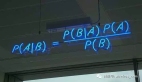
貝葉斯推理三種方法:MCMC 、HMC和SBI

開發 測試
對許多人來說,貝葉斯統計仍然有些陌生。因為貝葉斯統計中會有一些主觀的先驗,在沒有測試數據的支持下了解他的理論還是有一些困難的。

對許多人來說,貝葉斯統計仍然有些陌生。因為貝葉斯統計中會有一些主觀的先驗,在沒有測試數據的支持下了解他的理論還是有一些困難的。本文整理的是作者最近在普林斯頓的一個研討會上做的演講幻燈片,這樣可以闡明為什么貝葉斯方法不僅在邏輯上是合理的,而且使用起來也很簡單。這里將以三種不同的方式實現相同的推理問題。

圖片

數據

我們的例子是在具有傾斜背景的噪聲數據中找到峰值的問題,這可能出現在粒子物理學和其他多分量事件過程中。

首先生成數據:

%matplotlib inline
%config InlineBackend.figure_format = 'svg'
import matplotlib.pyplot as plt
import numpy as np

def signal(theta, x):
l, m, s, a, b = theta

peak = l * np.exp(-(m-x)**2 / (2*s**2))
background = a + b*x

return peak + background

def plot_results(x, y, y_err, samples=None, predictions=None):
fig = plt.figure()
ax = fig.gca()
ax.errorbar(x, y, yerr=y_err, fmt=".k", capsize=0, label="Data")
x0 = np.linspace(-0.2, 1.2, 100)
ax.plot(x0, signal(theta, x0), "r", label="Truth", zorder=0)

if samples is not None:
inds = np.random.randint(len(samples), size=50)
for i,ind in enumerate(inds):
theta_ = samples[ind]
if i==0:
label='Posterior'
else:
label=None
ax.plot(x0, signal(theta_, x0), "C0", alpha=0.1, zorder=-1, label=label)
elif predictions is not None:
for i, pred in enumerate(predictions):
if i==0:
label='Posterior'
else:
label=None
ax.plot(x0, pred, "C0", alpha=0.1, zorder=-1, label=label)

ax.legend(frameon=False)
ax.set_xlabel("x")
ax.set_ylabel("y")
fig.tight_layout()
plt.close();
return fig

# random x locations
N = 40
np.random.seed(0)
x = np.random.rand(N)

# evaluate the true model at the given x values
theta = [1, 0.5, 0.1, -0.1, 0.4]
y = signal(theta, x)

# add heteroscedastic Gaussian uncertainties only in y direction
y_err = np.random.uniform(0.05, 0.25, size=N)
y = y + np.random.normal(0, y_err)

# plot
plot_results(x, y, y_err)

圖片

有了數據我們可以介紹三種方法了。

馬爾可夫鏈蒙特卡羅 Markov Chain Monte Carlo

emcee是用純python實現的,它只需要評估后驗的對數作為參數θ的函數。這里使用對數很有用,因為它使指數分布族的分析評估更容易,并且因為它更好地處理通常出現的非常小的數字。

import emcee

def log_likelihood(theta, x, y, yerr):
y_model = signal(theta, x)
chi2 = (y - y_model)**2 / (yerr**2)
return np.sum(-chi2 / 2)

def log_prior(theta):
if all(theta > -2) and (theta[2] > 0) and all(theta < 2):
return 0
return -np.inf

def log_posterior(theta, x, y, yerr):
lp = log_prior(theta)
if np.isfinite(lp):
lp += log_likelihood(theta, x, y, yerr)
return lp


# create a small ball around the MLE the initialize each walker
nwalkers, ndim = 30, 5
theta_guess = [0.5, 0.6, 0.2, -0.2, 0.1]
pos = theta_guess + 1e-4 * np.random.randn(nwalkers, ndim)

# run emcee
sampler = emcee.EnsembleSampler(nwalkers, ndim, log_posterior, args=(x, y, y_err))
sampler.run_mcmc(pos, 10000, progress=True);

結果如下:

100%|██████████| 10000/10000 [00:05<00:00, 1856.57it/s]

我們應該始終檢查生成的鏈,確定burn-in period,并且需要人肉觀察平穩性:

fig, axes = plt.subplots(ndim, sharex=True)
mcmc_samples = sampler.get_chain()
labels = ["l", "m", "s", "a", "b"]
for i in range(ndim):
ax = axes[i]
ax.plot(mcmc_samples[:, :, i], "k", alpha=0.3, rasterized=True)
ax.set_xlim(0, 1000)
ax.set_ylabel(labels[i])

axes[-1].set_xlabel("step number");

現在我們需要細化鏈因為我們的樣本是相關的。這里有一個方法來計算每個參數的自相關,我們可以將所有的樣本結合起來:

tau = sampler.get_autocorr_time()
print("Autocorrelation time:", tau)
mcmc_samples = sampler.get_chain(discard=300, thin=np.int32(np.max(tau)/2), flat=True)
print("Remaining samples:", mcmc_samples.shape)

#結果
Autocorrelation time: [122.51626866 75.87228105 137.195509 54.63572513 79.0331587 ]
Remaining samples: (4260, 5)

emcee 的創建者 Dan Foreman-Mackey 還提供了這一有用的包corner來可視化樣本:

import corner

corner.corner(mcmc_samples, labels=labels, truths=theta);

圖片

雖然后驗樣本是推理的主要依據,但參數輪廓本身卻很難解釋。但是使用樣本來生成新數據則要簡單得多,因為這個可視化我們對數據空間有更多的理解。以下是來自50個隨機樣本的模型評估:

plot_results(x, y, y_err, samples=mcmc_samples)

圖片

哈密爾頓蒙特卡洛 Hamiltonian Monte Carlo

梯度在高維設置中提供了更多指導。 為了實現一般推理,我們需要一個框架來計算任意概率模型的梯度。 這里關鍵的本部分是自動微分,我們需要的是可以跟蹤參數的各種操作路徑的計算框架。 為了簡單起見,我們使用的框架是 jax。因為一般情況下在 numpy 中實現的函數都可以在 jax 中的進行類比的替換,而jax可以自動計算函數的梯度。

另外還需要計算概率分布梯度的能力。有幾種概率編程語言中可以實現,這里我們選擇了 NumPyro。 讓我們看看如何進行自動推理:

import jax.numpy as jnp
import jax.random as random
import numpyro
import numpyro.distributions as dist
from numpyro.infer import MCMC, NUTS

def model(x, y=None, y_err=0.1):

# define parameters (incl. prior ranges)
l = numpyro.sample('l', dist.Uniform(-2, 2))
m = numpyro.sample('m', dist.Uniform(-2, 2))
s = numpyro.sample('s', dist.Uniform(0, 2))
a = numpyro.sample('a', dist.Uniform(-2, 2))
b = numpyro.sample('b', dist.Uniform(-2, 2))

# implement the model
# needs jax numpy for differentiability here
peak = l * jnp.exp(-(m-x)**2 / (2*s**2))
background = a + b*x
y_model = peak + background

# notice that we clamp the outcome of this sampling to the observation y
numpyro.sample('obs', dist.Normal(y_model, y_err), obs=y)

# need to split the key for jax's random implementation
rng_key = random.PRNGKey(0)
rng_key, rng_key_ = random.split(rng_key)

# run HMC with NUTS
kernel = NUTS(model, target_accept_prob=0.9)
mcmc = MCMC(kernel, num_warmup=1000, num_samples=3000)
mcmc.run(rng_key_, x=x, y=y, y_err=y_err)
mcmc.print_summary()

#結果如下:
sample: 100%|██████████| 4000/4000 [00:03<00:00, 1022.99it/s, 17 steps of size 2.08e-01. acc. prob=0.94]


mean std median 5.0% 95.0% n_eff r_hat
a -0.13 0.05 -0.13 -0.22 -0.05 1151.15 1.00
b 0.46 0.07 0.46 0.36 0.57 1237.44 1.00
l 0.98 0.05 0.98 0.89 1.06 1874.34 1.00
m 0.50 0.01 0.50 0.49 0.51 1546.56 1.01
s 0.11 0.01 0.11 0.09 0.12 1446.08 1.00

Number of divergences: 0

還是使用corner可視化Numpyro的mcmc結構:

圖片

因為我們已經實現了整個概率模型(與emcee相反,我們只實現后驗),所以可以直接從樣本中創建后驗預測。下面,我們將噪聲設置為零,以得到純模型的無噪聲表示:

from numpyro.infer import Predictive

# make predictions from posterior
hmc_samples = mcmc.get_samples()
predictive = Predictive(model, hmc_samples)
# need to set noise to zero
# since the full model contains noise contribution
predictions = predictive(rng_key_, x=x0, y_err=0)['obs']

# select 50 predictions to show
inds = random.randint(rng_key_, (50,) , 0, mcmc.num_samples)
predictions = predictions[inds]

plot_results(x, y, y_err, predictions=predictions)

圖片

基于仿真的推理 Simulation-based Inference

在某些情況下,我們不能或不想計算可能性。 所以我們只能一個得到一個仿真器(即學習輸入之間的映射 θ 和仿真器的輸出 D),這個仿真器可以形成似然或后驗的近似替代。 與產生無噪聲模型的傳統模擬案例的一個重要區別是,需要在模擬中添加噪聲并且噪聲模型應盡可能與觀測噪聲匹配。 否則我們無法區分由于噪聲引起的數據變化和參數變化引起的數據變化。

import torch
from sbi import utils as utils

low = torch.zeros(ndim)
low[3] = -1
high = 1*torch.ones(ndim)
high[0] = 2
prior = utils.BoxUniform(low=low, high=high)

def simulator(theta, x, y_err):

# signal model
l, m, s, a, b = theta
peak = l * torch.exp(-(m-x)**2 / (2*s**2))
background = a + b*x
y_model = peak + background

# add noise consistent with observations
y = y_model + y_err * torch.randn(len(x))

return y

讓我們來看看噪聲仿真器的輸出:

plt.errorbar(x, this_simulator(torch.tensor(theta)), yerr=y_err, fmt=".r", capsize=0)
plt.errorbar(x, y, yerr=y_err, fmt=".k", capsize=0)
plt.plot(x0, signal(theta, x0), "k", label="truth")

圖片

現在,我們使用 sbi 從這些模擬仿真中訓練神經后驗估計 (NPE)。

from sbi.inference.base import infer

this_simulator = lambda theta: simulator(theta, torch.tensor(x), torch.tensor(y_err))

posterior = infer(this_simulator, prior, method='SNPE', num_simulations=10000)

NPE使用條件歸一化流來學習如何在給定一些數據的情況下生成后驗分布:

Running 10000 simulations.:   0%|         | 0/10000 [00:00<?, ?it/s]
Neural network successfully converged after 172 epochs.

在推理時,以實際數據 y 為條件簡單地評估這個神經后驗:

sbi_samples = posterior.sample((10000,), x=torch.tensor(y))
sbi_samples = sbi_samples.detach().numpy()

可以看到速度非常快幾乎不需要什么時間。

Drawing 10000 posterior samples:   0%|         | 0/10000 [00:00<?, ?it/s]

然后我們再次可視化后驗樣本:

corner.corner(sbi_samples, labels=labels, truths=theta);

圖片

plot_results(x, y, y_err, samples=sbi_samples)

圖片

可以看到仿真SBI的的結果不如 MCMC 和 HMC 的結果。 但是它們可以通過對更多模擬進行訓練以及通過調整網絡的架構來改進(雖然并不確定改完后就會有提高)。

但是我們可以看到即使在沒有擬然性的情況下,SBI 也可以進行近似貝葉斯推理。

責任編輯:華軒 來源: DeepHub IMBA
相關推薦

2017-08-07 13:02:32

全棧必備貝葉斯

2009-07-08 12:56:32

編寫Servlet

2023-02-24 16:45:02

2022-07-13 16:06:16

Python參數代碼

2009-12-11 18:49:39

預算編制博科資訊

2024-11-15 07:00:00

Python發送郵件

2011-04-18 15:32:45

游戲測試測試方法軟件測試

2010-09-14 15:10:49

CSS注釋

2023-08-14 17:58:13

RequestHTTP請求

2011-06-10 10:43:12

Ubuntu應用安裝

2009-06-23 10:45:18

Hibernate支持

2013-01-04 15:47:54

Android開發平鋪UI設計

2017-06-12 06:31:55

深度學習貝葉斯算法

2021-07-13 12:31:27

IT組織改進首席技術官

2023-05-16 16:07:07

大數據數據管理工具

2009-07-23 15:17:54

JDBC連接Acces

2016-09-09 13:07:56

CentOSJDKLinux

2010-07-29 09:56:45

Flex數據庫

2023-09-25 15:08:43

Python方離群值

2021-09-10 18:09:42

SQL注入漏洞網絡攻擊
點贊
收藏

51CTO技術棧公眾號

主站蜘蛛池模板: 在线观看成人精品 | 国产色片 | 男女啪啪网址 | 日韩av一区二区在线观看 | 精品国产精品一区二区夜夜嗨 | 国产欧美日韩视频 | 成人精品一区 | 九一视频在线观看 | 99精品一区二区 | 国产一区二区三区视频在线观看 | 亚洲美女一区二区三区 | 中文字幕成人av | 一区二区三区在线免费观看 | 婷婷五月色综合香五月 | 国产精品久久亚洲 | 成年人在线播放 | 亚洲精品乱码久久久久久蜜桃 | 亚洲国产成人在线视频 | 国产一区二区三区 | 国产成人免费视频网站高清观看视频 | 日韩欧美视频免费在线观看 | 一区二区精品 | 国产免费观看一级国产 | 黄色av网站在线观看 | 91国产在线视频在线 | 成人午夜激情 | 国产成人av一区二区三区 | 亚洲成人av一区二区 | www.亚洲免费 | 盗摄精品av一区二区三区 | 欧美在线观看一区 | 国产特一级黄色片 | 国产精品国产三级国产aⅴ中文 | 中文字幕亚洲视频 | 色秀网站 | 欧美一区久久 | 久久精品国产精品青草 | 精品国产乱码久久久久久蜜柚 | tube国产| 中文字幕日本一区二区 | 黄色片在线观看网址 |