深度學習神經網絡的預測間隔
預測間隔為回歸問題的預測提供了不確定性度量。
例如,95%的預測間隔表示100次中的95次,真實值將落在該范圍的下限值和上限值之間。這不同于可能表示不確定性區間中心的簡單點預測。沒有用于計算深度學習神經網絡關于回歸預測建模問題的預測間隔的標準技術。但是,可以使用一組模型來估計快速且骯臟的預測間隔,這些模型又提供了點預測的分布,可以從中計算間隔。
在本教程中,您將發現如何計算深度學習神經網絡的預測間隔。完成本教程后,您將知道:
- 預測間隔為回歸預測建模問題提供了不確定性度量。
- 如何在標準回歸問題上開發和評估簡單的多層感知器神經網絡。
- 如何使用神經網絡模型集成來計算和報告預測間隔。
教程概述
本教程分為三個部分:他們是:
- 預測間隔
- 回歸神經網絡
- 神經網絡預測間隔
預測間隔
通常,用于回歸問題的預測模型(即預測數值)進行點預測。這意味著他們可以預測單個值,但不能提供任何有關該預測的不確定性的指示。根據定義,預測是估計值或近似值,并且包含一些不確定性。不確定性來自模型本身的誤差和輸入數據中的噪聲。該模型是輸入變量和輸出變量之間關系的近似值。預測間隔是對預測不確定性的量化。它為結果變量的估計提供了概率上限和下限。
預測間隔是在預測數量的回歸模型中進行預測或預測時最常使用的時間間隔。預測間隔圍繞模型所做的預測,并希望覆蓋真實結果的范圍。有關一般的預測間隔的更多信息,請參見教程:
《機器學習的預測間隔》:
https://machinelearningmastery.com/prediction-intervals-for-machine-learning/
既然我們熟悉了預測間隔,那么我們可以考慮如何計算神經網絡的間隔。首先定義一個回歸問題和一個神經網絡模型來解決這個問題。
回歸神經網絡
在本節中,我們將定義回歸預測建模問題和神經網絡模型來解決該問題。首先,讓我們介紹一個標準回歸數據集。我們將使用住房數據集。住房數據集是一個標準的機器學習數據集,包括506行數據,其中包含13個數字輸入變量和一個數字目標變量。
使用具有三個重復的重復分層10倍交叉驗證的測試工具,一個樸素的模型可以實現約6.6的平均絕對誤差(MAE)。在大約1.9的相同測試工具上,性能最高的模型可以實現MAE。這為該數據集提供了預期性能的界限。該數據集包括根據美國波士頓市房屋郊區的詳細信息來預測房價。
房屋數據集(housing.csv):
https://raw.githubusercontent.com/jbrownlee/Datasets/master/housing.csv
房屋描述(房屋名稱):
https://raw.githubusercontent.com/jbrownlee/Datasets/master/housing.names
無需下載數據集;作為我們工作示例的一部分,我們將自動下載它。
下面的示例將數據集下載并加載為Pandas DataFrame,并概述了數據集的形狀和數據的前五行。
- # load and summarize the housing dataset
- from pandas import read_csv
- from matplotlib import pyplot
- # load dataset
- url = 'https://raw.githubusercontent.com/jbrownlee/Datasets/master/housing.csv'
- dataframe = read_csv(url, header=None)
- # summarize shape
- print(dataframe.shape)
- # summarize first few lines
- print(dataframe.head())
運行示例將確認506行數據和13個輸入變量以及一個數字目標變量(總共14個)。我們還可以看到所有輸入變量都是數字。
- (506, 14)
- 0 1 2 3 4 5 ... 8 9 10 11 12 13
- 0 0.00632 18.0 2.31 0 0.538 6.575 ... 1 296.0 15.3 396.90 4.98 24.0
- 1 0.02731 0.0 7.07 0 0.469 6.421 ... 2 242.0 17.8 396.90 9.14 21.6
- 2 0.02729 0.0 7.07 0 0.469 7.185 ... 2 242.0 17.8 392.83 4.03 34.7
- 3 0.03237 0.0 2.18 0 0.458 6.998 ... 3 222.0 18.7 394.63 2.94 33.4
- 4 0.06905 0.0 2.18 0 0.458 7.147 ... 3 222.0 18.7 396.90 5.33 36.2
- [5 rows x 14 columns]
接下來,我們可以準備用于建模的數據集。首先,可以將數據集拆分為輸入和輸出列,然后可以將行拆分為訓練和測試數據集。在這種情況下,我們將使用約67%的行來訓練模型,而其余33%的行用于估計模型的性能。
- # split into input and output values
- X, y = values[:,:-1], values[:,-1]
- # split into train and test sets
- X_train, X_test, y_train, y_test = train_test_split(X, y, train_size=0.67)
您可以在本教程中了解有關訓練測試拆分的更多信息:訓練測試拆分以評估機器學習算法然后,我們將所有輸入列(變量)縮放到0-1范圍,稱為數據歸一化,這在使用神經網絡模型時是一個好習慣。
- # scale input data
- scaler = MinMaxScaler()
- scaler.fit(X_train)
- X_train = scaler.transform(X_train)
- X_test = scaler.transform(X_test)
您可以在本教程中了解有關使用MinMaxScaler標準化輸入數據的更多信息:《如何在Python中使用StandardScaler和MinMaxScaler轉換 》:
https://machinelearningmastery.com/standardscaler-and-minmaxscaler-transforms-in-python/
下面列出了準備用于建模的數據的完整示例。
- # load and prepare the dataset for modeling
- from pandas import read_csv
- from sklearn.model_selection import train_test_split
- from sklearn.preprocessing import MinMaxScaler
- # load dataset
- url = 'https://raw.githubusercontent.com/jbrownlee/Datasets/master/housing.csv'
- dataframe = read_csv(url, header=None)
- values = dataframe.values
- # split into input and output values
- X, y = values[:,:-1], values[:,-1]
- # split into train and test sets
- X_train, X_test, y_train, y_test = train_test_split(X, y, train_size=0.67)
- # scale input data
- scaler = MinMaxScaler()
- scaler.fit(X_train)
- X_train = scaler.transform(X_train)
- X_test = scaler.transform(X_test)
- # summarize
- print(X_train.shape, X_test.shape, y_train.shape, y_test.shape)
運行示例像以前一樣加載數據集,然后將列拆分為輸入和輸出元素,將行拆分為訓練集和測試集,最后將所有輸入變量縮放到[0,1]范圍。列印了訓練圖和測試集的形狀,顯示我們有339行用于訓練模型,有167行用于評估模型。
- (339, 13) (167, 13) (339,) (167,)
接下來,我們可以在數據集中定義,訓練和評估多層感知器(MLP)模型。我們將定義一個簡單的模型,該模型具有兩個隱藏層和一個預測數值的輸出層。我們將使用ReLU激活功能和“ he”權重初始化,這是一個好習慣。經過一些反復試驗后,選擇了每個隱藏層中的節點數。
- # define neural network model
- features = X_train.shape[1]
- model = Sequential()
- model.add(Dense(20, kernel_initializer='he_normal', activation='relu', input_dim=features))
- model.add(Dense(5, kernel_initializer='he_normal', activation='relu'))
- model.add(Dense(1))
我們將使用具有接近默認學習速率和動量值的高效亞當版隨機梯度下降法,并使用均方誤差(MSE)損失函數(回歸預測建模問題的標準)擬合模型。
- # compile the model and specify loss and optimizer
- opt = Adam(learning_rate=0.01, beta_1=0.85, beta_2=0.999)
- model.compile(optimizer=opt, loss='mse')
您可以在本教程中了解有關Adam優化算法的更多信息:
《從頭開始編寫代碼Adam梯度下降優化》
https://machinelearningmastery.com/adam-optimization-from-scratch/
然后,該模型將適合300個紀元,批處理大小為16個樣本。經過一番嘗試和錯誤后,才選擇此配置。
- # fit the model on the training dataset
- model.fit(X_train, y_train, verbose=2, epochs=300, batch_size=16)
您可以在本教程中了解有關批次和紀元的更多信息:
《神經網絡中批次與時期之間的差異》
https://machinelearningmastery.com/difference-between-a-batch-and-an-epoch/
最后,該模型可用于在測試數據集上進行預測,我們可以通過將預測值與測試集中的預期值進行比較來評估預測,并計算平均絕對誤差(MAE),這是模型性能的一種有用度量。
- # make predictions on the test set
- yhat = model.predict(X_test, verbose=0)
- # calculate the average error in the predictions
- mae = mean_absolute_error(y_test, yhat)
- print('MAE: %.3f' % mae)
完整實例如下:
- # train and evaluate a multilayer perceptron neural network on the housing regression dataset
- from pandas import read_csv
- from sklearn.model_selection import train_test_split
- from sklearn.metrics import mean_absolute_error
- from sklearn.preprocessing import MinMaxScaler
- from tensorflow.keras.models import Sequential
- from tensorflow.keras.layers import Dense
- from tensorflow.keras.optimizers import Adam
- # load dataset
- url = 'https://raw.githubusercontent.com/jbrownlee/Datasets/master/housing.csv'
- dataframe = read_csv(url, header=None)
- values = dataframe.values
- # split into input and output values
- X, y = values[:, :-1], values[:,-1]
- # split into train and test sets
- X_train, X_test, y_train, y_test = train_test_split(X, y, train_size=0.67, random_state=1)
- # scale input data
- scaler = MinMaxScaler()
- scaler.fit(X_train)
- X_train = scaler.transform(X_train)
- X_test = scaler.transform(X_test)
- # define neural network model
- features = X_train.shape[1]
- model = Sequential()
- model.add(Dense(20, kernel_initializer='he_normal', activation='relu', input_dim=features))
- model.add(Dense(5, kernel_initializer='he_normal', activation='relu'))
- model.add(Dense(1))
- # compile the model and specify loss and optimizer
- opt = Adam(learning_rate=0.01, beta_1=0.85, beta_2=0.999)
- model.compile(optimizer=opt, loss='mse')
- # fit the model on the training dataset
- model.fit(X_train, y_train, verbose=2, epochs=300, batch_size=16)
- # make predictions on the test set
- yhat = model.predict(X_test, verbose=0)
- # calculate the average error in the predictions
- mae = mean_absolute_error(y_test, yhat)
- print('MAE: %.3f' % mae)
運行示例將加載并準備數據集,在訓練數據集上定義MLP模型并將其擬合,并在測試集上評估其性能。
注意:由于算法或評估程序的隨機性,或者數值精度的差異,您的結果可能會有所不同。考慮運行該示例幾次并比較平均結果。
在這種情況下,我們可以看到該模型實現的平均絕對誤差約為2.3,這比樸素的模型要好,并且接近于最佳模型。
毫無疑問,通過進一步調整模型,我們可以達到接近最佳的性能,但這對于我們研究預測間隔已經足夠了。
- Epoch 296/300
- 22/22 - 0s - loss: 7.1741
- Epoch 297/300
- 22/22 - 0s - loss: 6.8044
- Epoch 298/300
- 22/22 - 0s - loss: 6.8623
- Epoch 299/300
- 22/22 - 0s - loss: 7.7010
- Epoch 300/300
- 22/22 - 0s - loss: 6.5374
- MAE: 2.300
接下來,讓我們看看如何使用住房數據集上的MLP模型計算預測間隔。
神經網絡預測間隔
在本節中,我們將使用上一節中開發的回歸問題和模型來開發預測間隔。
與像線性回歸這樣的線性方法(預測間隔計算很簡單)相比,像神經網絡這樣的非線性回歸算法的預測間隔計算具有挑戰性。沒有標準技術。有許多方法可以為神經網絡模型計算有效的預測間隔。我建議“更多閱讀”部分列出的一些論文以了解更多信息。
在本教程中,我們將使用一種非常簡單的方法,該方法具有很大的擴展空間。我將其稱為“快速且骯臟的”,因為它快速且易于計算,但有一定的局限性。它涉及擬合多個最終模型(例如10到30)。來自集合成員的點預測的分布然后用于計算點預測和預測間隔。
例如,可以將點預測作為來自集合成員的點預測的平均值,并且可以將95%的預測間隔作為與該平均值的1.96標準偏差。這是一個簡單的高斯預測間隔,盡管可以使用替代方法,例如點預測的最小值和最大值。或者,可以使用自舉方法在不同的自舉樣本上訓練每個合奏成員,并且可以將點預測的第2.5個百分點和第97.5個百分點用作預測間隔。
有關bootstrap方法的更多信息,請參見教程:
《Bootstrap方法的簡要介紹》
https://machinelearningmastery.com/a-gentle-introduction-to-the-bootstrap-method/
這些擴展保留為練習;我們將堅持簡單的高斯預測區間。
假設在上一部分中定義的訓練數據集是整個數據集,并且我們正在對該整個數據集訓練一個或多個最終模型。然后,我們可以在測試集上使用預測間隔進行預測,并評估該間隔在將來的有效性。
我們可以通過將上一節中開發的元素劃分為功能來簡化代碼。首先,讓我們定義一個函數,以加載和準備由URL定義的回歸數據集。
- # load and prepare the dataset
- def load_dataset(url):
- dataframe = read_csv(url, header=None)
- values = dataframe.values
- # split into input and output values
- X, y = values[:, :-1], values[:,-1]
- # split into train and test sets
- X_train, X_test, y_train, y_test = train_test_split(X, y, train_size=0.67, random_state=1)
- # scale input data
- scaler = MinMaxScaler()
- scaler.fit(X_train)
- X_train = scaler.transform(X_train)
- X_test = scaler.transform(X_test)
- return X_train, X_test, y_train, y_test
接下來,我們可以定義一個函數,該函數將在給定訓練數據集的情況下定義和訓練MLP模型,然后返回適合進行預測的擬合模型。
- # define and fit the model
- def fit_model(X_train, y_train):
- # define neural network model
- features = X_train.shape[1]
- model = Sequential()
- model.add(Dense(20, kernel_initializer='he_normal', activation='relu', input_dim=features))
- model.add(Dense(5, kernel_initializer='he_normal', activation='relu'))
- model.add(Dense(1))
- # compile the model and specify loss and optimizer
- opt = Adam(learning_rate=0.01, beta_1=0.85, beta_2=0.999)
- model.compile(optimizer=opt, loss='mse')
- # fit the model on the training dataset
- model.fit(X_train, y_train, verbose=0, epochs=300, batch_size=16)
- return model
我們需要多個模型來進行點預測,這些模型將定義點預測的分布,從中可以估計間隔。
因此,我們需要在訓練數據集上擬合多個模型。每個模型必須不同,以便做出不同的預測。在訓練MLP模型具有隨機性,隨機初始權重以及使用隨機梯度下降優化算法的情況下,可以實現這一點。模型越多,點預測將更好地估計模型的功能。我建議至少使用10種型號,而超過30種型號可能不會帶來太多好處。下面的函數適合模型的整體,并將其存儲在返回的列表中。出于興趣,還對測試集評估了每個擬合模型,并在擬合每個模型后報告了該測試集。我們希望每個模型在保持測試集上的估計性能會略有不同,并且報告的分數將有助于我們確認這一期望。
- # fit an ensemble of models
- def fit_ensemble(n_members, X_train, X_test, y_train, y_test):
- ensemble = list()
- for i in range(n_members):
- # define and fit the model on the training set
- model = fit_model(X_train, y_train)
- # evaluate model on the test set
- yhat = model.predict(X_test, verbose=0)
- mae = mean_absolute_error(y_test, yhat)
- print('>%d, MAE: %.3f' % (i+1, mae))
- # store the model
- ensemble.append(model)
- return ensemble
最后,我們可以使用訓練有素的模型集合進行點預測,可以將其總結為一個預測區間。
下面的功能實現了這一點。首先,每個模型對輸入數據進行點預測,然后計算95%的預測間隔,并返回該間隔的下限值,平均值和上限值。
該函數被設計為將單行作為輸入,但是可以很容易地適應于多行。
- # make predictions with the ensemble and calculate a prediction interval
- def predict_with_pi(ensemble, X):
- # make predictions
- yhat = [model.predict(X, verbose=0) for model in ensemble]
- yhat = asarray(yhat)
- # calculate 95% gaussian prediction interval
- interval = 1.96 * yhat.std()
- lower, upper = yhat.mean() - interval, yhat.mean() + interval
- return lower, yhat.mean(), upper
最后,我們可以調用這些函數。首先,加載并準備數據集,然后定義并擬合集合。
- # load dataset
- url = 'https://raw.githubusercontent.com/jbrownlee/Datasets/master/housing.csv'
- X_train, X_test, y_train, y_test = load_dataset(url)
- # fit ensemble
- n_members = 30
- ensemble = fit_ensemble(n_members, X_train, X_test, y_train, y_test)
然后,我們可以使用測試集中的一行數據,并以預測間隔進行預測,然后報告結果。
我們還報告了預期的期望值,該期望值將在預測間隔內涵蓋(可能接近95%的時間;這并不完全準確,而是粗略的近似值)。
- # make predictions with prediction interval
- newX = asarray([X_test[0, :]])
- lower, mean, upper = predict_with_pi(ensemble, newX)
- print('Point prediction: %.3f' % mean)
- print('95%% prediction interval: [%.3f, %.3f]' % (lower, upper))
- print('True value: %.3f' % y_test[0])
綜上所述,下面列出了使用多層感知器神經網絡以預測間隔進行預測的完整示例。
- # prediction interval for mlps on the housing regression dataset
- from numpy import asarray
- from pandas import read_csv
- from sklearn.model_selection import train_test_split
- from sklearn.metrics import mean_absolute_error
- from sklearn.preprocessing import MinMaxScaler
- from tensorflow.keras.models import Sequential
- from tensorflow.keras.layers import Dense
- from tensorflow.keras.optimizers import Adam
- # load and prepare the dataset
- def load_dataset(url):
- dataframe = read_csv(url, header=None)
- values = dataframe.values
- # split into input and output values
- X, y = values[:, :-1], values[:,-1]
- # split into train and test sets
- X_train, X_test, y_train, y_test = train_test_split(X, y, train_size=0.67, random_state=1)
- # scale input data
- scaler = MinMaxScaler()
- scaler.fit(X_train)
- X_train = scaler.transform(X_train)
- X_test = scaler.transform(X_test)
- return X_train, X_test, y_train, y_test
- # define and fit the model
- def fit_model(X_train, y_train):
- # define neural network model
- features = X_train.shape[1]
- model = Sequential()
- model.add(Dense(20, kernel_initializer='he_normal', activation='relu', input_dim=features))
- model.add(Dense(5, kernel_initializer='he_normal', activation='relu'))
- model.add(Dense(1))
- # compile the model and specify loss and optimizer
- opt = Adam(learning_rate=0.01, beta_1=0.85, beta_2=0.999)
- model.compile(optimizer=opt, loss='mse')
- # fit the model on the training dataset
- model.fit(X_train, y_train, verbose=0, epochs=300, batch_size=16)
- return model
- # fit an ensemble of models
- def fit_ensemble(n_members, X_train, X_test, y_train, y_test):
- ensemble = list()
- for i in range(n_members):
- # define and fit the model on the training set
- model = fit_model(X_train, y_train)
- # evaluate model on the test set
- yhat = model.predict(X_test, verbose=0)
- mae = mean_absolute_error(y_test, yhat)
- print('>%d, MAE: %.3f' % (i+1, mae))
- # store the model
- ensemble.append(model)
- return ensemble
- # make predictions with the ensemble and calculate a prediction interval
- def predict_with_pi(ensemble, X):
- # make predictions
- yhat = [model.predict(X, verbose=0) for model in ensemble]
- yhat = asarray(yhat)
- # calculate 95% gaussian prediction interval
- interval = 1.96 * yhat.std()
- lower, upper = yhat.mean() - interval, yhat.mean() + interval
- return lower, yhat.mean(), upper
- # load dataset
- url = 'https://raw.githubusercontent.com/jbrownlee/Datasets/master/housing.csv'
- X_train, X_test, y_train, y_test = load_dataset(url)
- # fit ensemble
- n_members = 30
- ensemble = fit_ensemble(n_members, X_train, X_test, y_train, y_test)
- # make predictions with prediction interval
- newX = asarray([X_test[0, :]])
- lower, mean, upper = predict_with_pi(ensemble, newX)
- print('Point prediction: %.3f' % mean)
- print('95%% prediction interval: [%.3f, %.3f]' % (lower, upper))
- print('True value: %.3f' % y_test[0])
運行示例依次適合每個集合成員,并在保留測試集上報告其估計性能;最后,做出并預測一個具有預測間隔的預測。
注意:由于算法或評估程序的隨機性,或者數值精度的差異,您的結果可能會有所不同。考慮運行該示例幾次并比較平均結果。
在這種情況下,我們可以看到每個模型的性能略有不同,這證實了我們對模型確實有所不同的期望。
最后,我們可以看到該合奏以95%的預測間隔[26.287,34.822]進行了約30.5的點預測。我們還可以看到,真實值為28.2,并且間隔確實捕獲了該值,這非常好。
- >1, MAE: 2.259
- >2, MAE: 2.144
- >3, MAE: 2.732
- >4, MAE: 2.628
- >5, MAE: 2.483
- >6, MAE: 2.551
- >7, MAE: 2.505
- >8, MAE: 2.299
- >9, MAE: 2.706
- >10, MAE: 2.145
- >11, MAE: 2.765
- >12, MAE: 3.244
- >13, MAE: 2.385
- >14, MAE: 2.592
- >15, MAE: 2.418
- >16, MAE: 2.493
- >17, MAE: 2.367
- >18, MAE: 2.569
- >19, MAE: 2.664
- >20, MAE: 2.233
- >21, MAE: 2.228
- >22, MAE: 2.646
- >23, MAE: 2.641
- >24, MAE: 2.492
- >25, MAE: 2.558
- >26, MAE: 2.416
- >27, MAE: 2.328
- >28, MAE: 2.383
- >29, MAE: 2.215
- >30, MAE: 2.408
- Point prediction: 30.555
- 95% prediction interval: [26.287, 34.822]
- True value: 28.200
True value: 28.200