介紹

圖像分類是計算機視覺的最重要應用之一。它的應用范圍包括從自動駕駛汽車中的物體分類到醫療行業中的血細胞識別，從制造業中的缺陷物品識別到建立可以對戴口罩與否的人進行分類的系統。在所有這些行業中，圖像分類都以一種或另一種方式使用。他們是如何做到的呢？他們使用哪個框架？

你必須已閱讀很多有關不同深度學習框架（包括TensorFlow，PyTorch，Keras等）之間差異的信息。TensorFlow和PyTorch無疑是業內最受歡迎的框架。我相信你會發現無窮的資源來學習這些深度學習框架之間的異同。

在本文中，我們將了解如何在PyTorch和TensorFlow中建立基本的圖像分類模型。我們將從PyTorch和TensorFlow的簡要概述開始。然后，我們將使用MNIST手寫數字分類數據集，并在PyTorch和TensorFlow中使用CNN（卷積神經網絡）建立圖像分類模型。

這將是你的起點，然后你可以選擇自己喜歡的任何框架，也可以開始構建其他計算機視覺模型。

目錄

1. PyTorch概述
2. TensorFlow概述
3. 了解問題陳述：MNIST
4. 在PyTorch中實現卷積神經網絡（CNN）
5. 在TensorFlow中實施卷積神經網絡（CNN）

PyTorch概述

PyTorch在深度學習社區中越來越受歡迎，并且被深度學習從業者廣泛使用，PyTorch是一個提供Tensor計算的Python軟件包。此外，tensors是多維數組，就像NumPy的ndarrays也可以在GPU上運行一樣。

PyTorch的一個獨特功能是它使用動態計算圖。PyTorch的Autograd軟件包從張量生成計算圖并自動計算梯度。而不是具有特定功能的預定義圖形。

PyTorch為我們提供了一個框架，可以隨時隨地構建計算圖，甚至在運行時進行更改。特別是，對于我們不知道創建神經網絡需要多少內存的情況，這很有用。

你可以使用PyTorch應對各種深度學習挑戰。以下是一些挑戰：

1. 圖像（檢測，分類等）
2. 文字（分類，生成等）
3. 強化學習

TensorFlow概述

TensorFlow由Google Brain團隊的研究人員和工程師開發。它與深度學習領域最常用的軟件庫相距甚遠（盡管其他軟件庫正在迅速追趕）。

TensorFlow如此受歡迎的最大原因之一是它支持多種語言來創建深度學習模型，例如Python，C ++和R。它提供了詳細的文檔和指南的指導。

TensorFlow包含許多組件。以下是兩個杰出的代表：

1. TensorBoard：使用數據流圖幫助有效地可視化數據
2. TensorFlow：對于快速部署新算法/實驗非常有用

TensorFlow當前正在運行2.0版本，該版本于2019年9月正式發布。我們還將在2.0版本中實現CNN。

我希望你現在對PyTorch和TensorFlow都有基本的了解。現在，讓我們嘗試使用這兩個框架構建深度學習模型并了解其內部工作。在此之前，讓我們首先了解我們將在本文中解決的問題陳述。

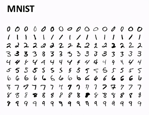
了解問題陳述：MNIST

在開始之前，讓我們了解數據集。在本文中，我們將解決流行的MNIST問題。這是一個數字識別任務，其中我們必須將手寫數字的圖像分類為0到9這10個類別之一。

在MNIST數據集中，我們具有從各種掃描的文檔中獲取的數字圖像，尺寸經過標準化并居中。隨后，每個圖像都是28 x 28像素的正方形（總計784像素）。數據集的標準拆分用于評估和比較模型，其中60,000張圖像用于訓練模型，而單獨的10,000張圖像集用于測試模型。

現在，我們也了解了數據集。因此，讓我們在PyTorch和TensorFlow中使用CNN構建圖像分類模型。我們將從PyTorch中的實現開始。我們將在google colab中實現這些模型，該模型提供免費的GPU以運行這些深度學習模型。

在PyTorch中實現卷積神經網絡（CNN）

讓我們首先導入所有庫：

# importing the libraries 
import numpy as np 
import torch 
import torchvision 
import matplotlib.pyplot as plt 
from time import time 
from torchvision import datasets, transforms 
from torch import nn, optim 

我們還要在Google colab上檢查PyTorch的版本：

# version of pytorch 
print(torch.__version__) 

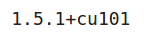
因此，我正在使用1.5.1版本的PyTorch。如果使用任何其他版本，則可能會收到一些警告或錯誤，因此你可以更新到此版本的PyTorch。我們將對圖像執行一些轉換，例如對像素值進行歸一化，因此，讓我們也定義這些轉換：

# transformations to be applied on images 
transform = transforms.Compose([transforms.ToTensor(), 
                              transforms.Normalize((0.5,), (0.5,)), 
                              ]) 

現在，讓我們加載MNIST數據集的訓練和測試集：

# defining the training and testing set 
trainset = datasets.MNIST('./data', download=True, train=True, transform=transform) 
testset = datasets.MNIST('./', download=True, train=False, transform=transform) 

接下來，我定義了訓練和測試加載器，這將幫助我們分批加載訓練和測試集。我將批量大小定義為64：

# defining trainloader and testloader 
trainloader = torch.utils.data.DataLoader(trainset, batch_size=64, shuffle=True) 
testloader = torch.utils.data.DataLoader(testset, batch_size=64, shuffle=True) 

首先讓我們看一下訓練集的摘要：

# shape of training data 
dataiter = iter(trainloader) 
images, labels = dataiter.next() 
 
print(images.shape) 
print(labels.shape) 

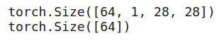
因此，在每個批次中，我們有64個圖像，每個圖像的大小為28,28，并且對于每個圖像，我們都有一個相應的標簽。讓我們可視化訓練圖像并查看其外觀：

# visualizing the training images 
plt.imshow(images[0].numpy().squeeze(), cmap='gray') 

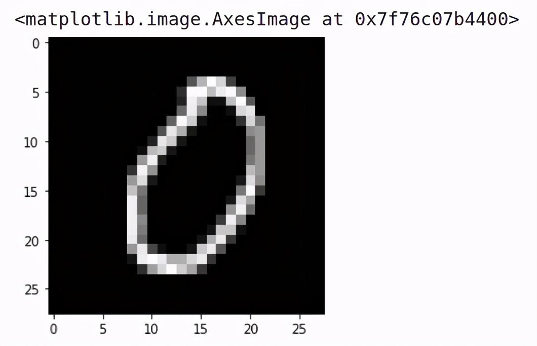
它是數字0的圖像。類似地，讓我們可視化測試集圖像：

# shape of validation data 
dataiter = iter(testloader) 
images, labels = dataiter.next() 
 
print(images.shape) 
print(labels.shape) 

在測試集中，我們也有大小為64的批次。現在讓我們定義架構

定義模型架構

我們將在這里使用CNN模型。因此，讓我們定義并訓練該模型：

# defining the model architecture 
class Net(nn.Module):    
  def __init__(self): 
      super(Net, self).__init__() 
 
      self.cnn_layers = nn.Sequential( 
          # Defining a 2D convolution layer 
          nn.Conv2d(1, 4, kernel_size=3, stride=1, padding=1), 
          nn.BatchNorm2d(4), 
          nn.ReLU(inplace=True), 
          nn.MaxPool2d(kernel_size=2, stride=2), 
          # Defining another 2D convolution layer 
          nn.Conv2d(4, 4, kernel_size=3, stride=1, padding=1), 
          nn.BatchNorm2d(4), 
          nn.ReLU(inplace=True), 
          nn.MaxPool2d(kernel_size=2, stride=2), 
      ) 
 
      self.linear_layers = nn.Sequential( 
          nn.Linear(4 * 7 * 7, 10) 
      ) 
 
  # Defining the forward pass     
  def forward(self, x): 
      x = self.cnn_layers(x) 
      x = x.view(x.size(0), -1) 
      x = self.linear_layers(x) 
      return x 

我們還定義優化器和損失函數，然后我們將看一下該模型的摘要：

# defining the model 
model = Net() 
# defining the optimizer 
optimizer = optim.Adam(model.parameters(), lr=0.01) 
# defining the loss function 
criterion = nn.CrossEntropyLoss() 
# checking if GPU is available 
if torch.cuda.is_available(): 
    model = model.cuda() 
    criterion = criterion.cuda() 
 
print(model) 

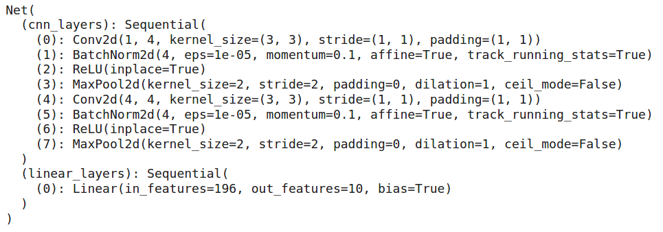
因此，我們有2個卷積層，這將有助于從圖像中提取特征。這些卷積層的特征傳遞到完全連接的層，該層將圖像分類為各自的類別。現在我們的模型架構已準備就緒，讓我們訓練此模型十個時期：

for i in range(10): 
    running_loss = 0 
    for images, labels in trainloader: 
 
        if torch.cuda.is_available(): 
          images = images.cuda() 
          labels = labels.cuda() 
 
        # Training pass 
        optimizer.zero_grad() 
 
        output = model(images) 
        loss = criterion(output, labels) 
 
        #This is where the model learns by backpropagating 
        loss.backward() 
 
        #And optimizes its weights here 
        optimizer.step() 
 
        running_loss += loss.item() 
    else: 
        print("Epoch {} - Training loss: {}".format(i+1, running_loss/len(trainloader))) 

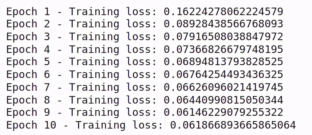
你會看到訓練隨著時期的增加而減少。這意味著我們的模型是從訓練集中學習模式。讓我們在測試集上檢查該模型的性能：

# getting predictions on test set and measuring the performance 
correct_count, all_count = 0, 0 
for images,labels in testloader: 
  for i in range(len(labels)): 
    if torch.cuda.is_available(): 
        images = images.cuda() 
        labels = labels.cuda() 
    img = images[i].view(1, 1, 28, 28) 
    with torch.no_grad(): 
        logps = model(img) 
 
 
    ps = torch.exp(logps) 
    probab = list(ps.cpu()[0]) 
    pred_label = probab.index(max(probab)) 
    true_label = labels.cpu()[i] 
    if(true_label == pred_label): 
      correct_count += 1 
    all_count += 1 
 
print("Number Of Images Tested =", all_count) 
print("\nModel Accuracy =", (correct_count/all_count)) 

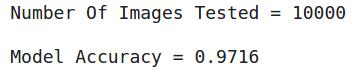
因此，我們總共測試了10000張圖片，并且該模型在預測測試圖片的標簽方面的準確率約為96％。

這是你可以在PyTorch中構建卷積神經網絡的方法。在下一節中，我們將研究如何在TensorFlow中實現相同的體系結構。

在TensorFlow中實施卷積神經網絡（CNN）

現在，讓我們在TensorFlow中使用卷積神經網絡解決相同的MNIST問題。與往常一樣，我們將從導入庫開始：

# importing the libraries 
import tensorflow as tf 
 
from tensorflow.keras import datasets, layers, models 
from tensorflow.keras.utils import to_categorical 
import matplotlib.pyplot as plt 

檢查一下我們正在使用的TensorFlow的版本：

# version of tensorflow 
print(tf.__version__) 

因此，我們正在使用TensorFlow的2.2.0版本。現在讓我們使用tensorflow.keras的數據集類加載MNIST數據集：

(train_images, train_labels), (test_images, test_labels) = datasets.mnist.load_data(path='mnist.npz') 
# Normalize pixel values to be between 0 and 1 
train_images, test_images = train_images / 255.0, test_images / 255.0 

在這里，我們已經加載了訓練以及MNIST數據集的測試集。此外，我們已經將訓練和測試圖像的像素值標準化了。接下來，讓我們可視化來自數據集的一些圖像：

# visualizing a few images 
plt.figure(figsize=(10,10)) 
for i in range(9): 
    plt.subplot(3,3,i+1) 
    plt.xticks([]) 
    plt.yticks([]) 
    plt.grid(False) 
    plt.imshow(train_images[i], cmap='gray') 
plt.show() 

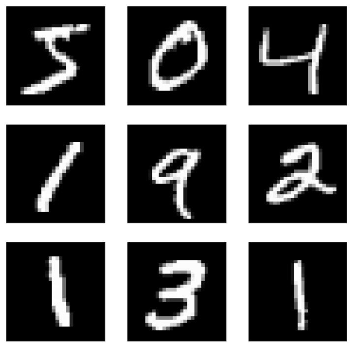
這就是我們的數據集的樣子。我們有手寫數字的圖像。再來看一下訓練和測試集的形狀：

# shape of the training and test set 
(train_images.shape, train_labels.shape), (test_images.shape, test_labels.shape) 

因此，我們在訓練集中有60,000張28乘28的圖像，在測試集中有10,000張相同形狀的圖像。接下來，我們將調整圖像的大小，并一鍵編碼目標變量：

# reshaping the images 
train_images = train_images.reshape((60000, 28, 28, 1)) 
test_images = test_images.reshape((10000, 28, 28, 1)) 
 
# one hot encoding the target variable 
train_labels = to_categorical(train_labels) 
test_labels = to_categorical(test_labels) 

定義模型體系結構

現在，我們將定義模型的體系結構。我們將使用Pytorch中定義的相同架構。因此，我們的模型將是具有2個卷積層，以及最大池化層的組合，然后我們將有一個Flatten層，最后是一個有10個神經元的全連接層，因為我們有10個類。

# defining the model architecture 
model = models.Sequential() 
model.add(layers.Conv2D(4, (3, 3), activation='relu', input_shape=(28, 28, 1))) 
model.add(layers.MaxPooling2D((2, 2), strides=2)) 
model.add(layers.Conv2D(4, (3, 3), activation='relu')) 
model.add(layers.MaxPooling2D((2, 2), strides=2)) 
model.add(layers.Flatten()) 
model.add(layers.Dense(10, activation='softmax')) 

讓我們快速看一下該模型的摘要：

# summary of the model 
model.summary() 

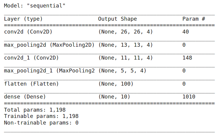
總而言之，我們有2個卷積層，2個最大池層，一個Flatten層和一個全連接層。模型中的參數總數為1198個。現在我們的模型已經準備好了，我們將編譯它：

# compiling the model 
model.compile(optimizer='adam', 
              loss='categorical_crossentropy', 
              metrics=['accuracy']) 

我們正在使用Adam優化器，你也可以對其進行更改。損失函數被設置為分類交叉熵，因為我們正在解決一個多類分類問題，并且度量標準是‘accuracy’。現在讓我們訓練模型10個時期

# training the model 
history = model.fit(train_images, train_labels, epochs=10, validation_data=(test_images, test_labels)) 

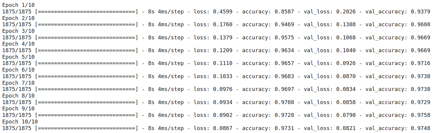
總而言之，最初，訓練損失約為0.46，經過10個時期后，訓練損失降至0.08。10個時期后的訓練和驗證準確性分別為97.31％和97.48％。

因此，這就是我們可以在TensorFlow中訓練CNN的方式。

尾注

總而言之，在本文中，我們首先研究了PyTorch和TensorFlow的簡要概述。然后我們了解了MNIST手寫數字分類的挑戰，最后，在PyTorch和TensorFlow中使用CNN（卷積神經網絡）建立了圖像分類模型。現在，我希望你熟悉這兩個框架。下一步，應對另一個圖像分類挑戰，并嘗試同時使用PyTorch和TensorFlow來解決。