這篇博文是用Python分析股市數據系列兩部中的第一部，內容基于我猶他大學 數學3900 (數據科學)的課程。在這些博文中，我會討論一些基礎知識。比如如何用pandas從雅虎財經獲得數據， 可視化股市數據，平局數指標的定義，設計移動平均交匯點分析移動平均線的方法，回溯測試， 基準分析法。最后一篇博文會包含問題以供練習。第一篇博文會包含平局數指標以及之前的內容。

注意：本文僅代表作者本人的觀點。文中的內容不應該被當做經濟建議。我不對文中代碼負責，取用者自己負責。

引言

金融業使用高等數學和統計已經有段時日。早在八十年代以前，銀行業和金融業被認為是“枯燥”的;投資銀行跟商業銀行是分開的,業界主要的任務是處理“簡單的”(跟當今相比)的金融職能，例如貸款。里根政府的減少調控和數學的應用，使該行業從枯燥的銀行業變為今天的模樣。在那之后，金融躋身科學，成為推動數學研究和發展的力量。例如數學上一個重大進展是布萊克-舒爾斯公式的推導。它被用來股票定價 (一份賦予股票持有者以一定的價格從股票發行者手中買入和賣出的合同)。但是, 不好的統計模型，包括布萊克-舒爾斯模型， 背負了部分導致2008金融危機的罵名。

近年來，計算機科學加入了高等數學的陣營，為金融和證券交易(為了盈利而進行的金融產品買入賣出行為)帶來了革命性的變化。如今交易主要由計算機來完成：算法能以人類難以達到的速度做出交易決策(參看光速的限制已經成為系統設計中的瓶頸)。機器學習和數據挖掘也被越來越廣泛的用到金融領域中，目測這個勢頭會保持下去。事實上很大一部分的算法交易都是高頻交易(HFT)。雖然算法比人工快，但這些技術還是很新，而且被應用在一個以不穩定，高風險著稱的領域。據一條被黑客曝光的白宮相關媒體推特表明HFT應該對2010 閃電式崩盤 and a 2013 閃電式崩盤 負責。

不過這節課不是關于如何利用不好的數學模型來摧毀證券市場。相反的，我將提供一些基本的Python工具來處理和分析股市數據。我會講到移動平均值，如何利用移動平均值來制定交易策略，如何制定進入和撤出股市的決策，記憶如何利用回溯測試來評估一個決策。

免責申明：這不是投資建議。同時我私人完全沒有交易經驗(文中相關的知識大部分來自我在鹽湖城社區大學參加的一個學期關于股市交易的課程)!這里僅僅是基本概念知識，不足以用于實際交易的股票。股票交易可以讓你受到損失(已有太多案例)，你要為自己的行為負責。

獲取并可視化股市數據

從雅虎金融獲取數據

在分析數據之前得先得到數據。股市數據可以從Yahoo! Finance、 Google Finance以及其他的地方拿到。同時，pandas包提供了輕松從以上網站獲取數據的方法。這節課我們使用雅虎金融的數據。

下面的代碼展示了如何直接創建一個含有股市數據的DataFrame。(更多關于遠程獲取數據的信息，點擊這里(http://pandas.pydata.org/pandas-docs/stable/remote_data.html))

import pandas as pd 
 
import pandas.io.data as web   # Package and modules for importing data; this code may change depending on pandas version 
 
import datetime 
 
  
 
# We will look at stock prices over the past year, starting at January 1, 2016 
 
start = datetime.datetime(2016,1,1) 
 
end = datetime.date.today() 
 
  
 
# Let's get Apple stock data; Apple's ticker symbol is AAPL 
 
# First argument is the series we want, second is the source ("yahoo" for Yahoo! Finance), third is the start date, fourth is the end date 
 
apple = web.DataReader("AAPL", "yahoo", start, end) 
 
  
 
type(apple)  

C:\Anaconda3\lib\site-packages\pandas\io\data.py:35: FutureWarning: 
 
The pandas.io.data module is moved to a separate package (pandas-datareader) and will be removed from pandas in a future version. 
 
After installing the pandas-datareader package (https://github.com/pydata/pandas-datareader), you can change the import ``from pandas.io import data, wb`` to ``from pandas_datareader import data, wb``. 
 
  FutureWarning) 
 
  
 
  
 
  
 
  
 
  
 
pandas.core.frame.DataFrame  

apple.head() 

讓我們簡單說一下數據內容。Open是當天的開始價格(不是前一天閉市的價格);high是股票當天的最高價;low是股票當天的最低價;close是閉市時間的股票價格。Volume指交易數量。Adjust close是根據法人行為調整之后的閉市價格。雖然股票價格基本上是由交易者決定的，stock splits (拆股。指上市公司將現有股票一拆為二，新股價格為原股的一半的行為)以及dividends(分紅。每一股的分紅)同樣也會影響股票價格，也應該在模型中被考慮到。

可視化股市數據

獲得數據之后讓我們考慮將其可視化。下面我會演示如何使用matplotlib包。值得注意的是appleDataFrame對象有一個plot()方法讓畫圖變得更簡單。 

import matplotlib.pyplot as plt   # Import matplotlib 
 
# This line is necessary for the plot to appear in a Jupyter notebook 
 
%matplotlib inline 
 
  
 
# Control the default size of figures in this Jupyter notebook 
 
%pylab inline 
 
  
 
pylab.rcParams['figure.figsize'] = (15, 9)   # Change the size of plots 
 
apple["Adj Close"].plot(grid = True) # Plot the adjusted closing price of AAPL  

Populating the interactive namespace from numpy and matplotlib 

線段圖是可行的，但是每一天的數據至少有四個變量(開市，股票最高價，股票最低價和閉市)，我們希望找到一種不需要我們畫四條不同的線就能看到這四個變量走勢的可視化方法。一般來說我們使用燭柱圖(也稱為日本陰陽燭圖表)來可視化金融數據，燭柱圖最早在18世紀被日本的稻米商人所使用。可以用matplotlib來作圖，但是需要費些功夫。

你們可以使用我實現的一個函數更容易地畫燭柱圖，它接受pandas的data frame作為數據來源。(程序基于這個例子, 你可以從這里找到相關函數的文檔。)

from matplotlib.dates import DateFormatter, WeekdayLocator,\ 
 
    DayLocator, MONDAY 
 
from matplotlib.finance import candlestick_ohlc 
 
def pandas_candlestick_ohlc(dat, stick = "day", otherseries = None): 
 
    """ 
 
    :param dat: pandas DataFrame object with datetime64 index, and float columns "Open", "High", "Low", and "Close", likely created via DataReader from "yahoo" 
 
    :param stick: A string or number indicating the period of time covered by a single candlestick. Valid string inputs include "day", "week", "month", and "year", ("day" default), and any numeric input indicates the number of trading days included in a period 
 
    :param otherseries: An iterable that will be coerced into a list, containing the columns of dat that hold other series to be plotted as lines 
 
    This will show a Japanese candlestick plot for stock data stored in dat, also plotting other series if passed. 
 
    """ 
 
    mondays = WeekdayLocator(MONDAY)        # major ticks on the mondays 
 
    alldays = DayLocator()              # minor ticks on the days 
 
    dayFormatter = DateFormatter('%d')      # e.g., 12 
 
    # Create a new DataFrame which includes OHLC data for each period specified by stick input 
 
    transdat = dat.loc[:,["Open", "High", "Low", "Close"]] 
 
    if (type(stick) == str): 
 
        if stick == "day": 
 
            plotdat = transdat 
 
            stick = 1 # Used for plotting 
 
        elif stick in ["week", "month", "year"]: 
 
            if stick == "week": 
 
                transdat["week"] = pd.to_datetime(transdat.index).map(lambda x: x.isocalendar()[1]) # Identify weeks 
 
            elif stick == "month": 
 
                transdat["month"] = pd.to_datetime(transdat.index).map(lambda x: x.month) # Identify months 
 
            transdat["year"] = pd.to_datetime(transdat.index).map(lambda x: x.isocalendar()[0]) # Identify years 
 
            grouped = transdat.groupby(list(set(["year",stick]))) # Group by year and other appropriate variable 
 
            plotdat = pd.DataFrame({"Open": [], "High": [], "Low": [], "Close": []}) # Create empty data frame containing what will be plotted 
 
            for name, group in grouped: 
 
                plotdat = plotdat.append(pd.DataFrame({"Open": group.iloc[0,0], 
 
                                            "High": max(group.High), 
 
                                            "Low": min(group.Low), 
 
                                            "Close": group.iloc[-1,3]}, 
 
                                           index = [group.index[0]])) 
 
            if stick == "week": stick = 5 
 
            elif stick == "month": stick = 30 
 
            elif stick == "year": stick = 365 
 
    elif (type(stick) == int and stick >= 1): 
 
        transdat["stick"] = [np.floor(i / stick) for i in range(len(transdat.index))] 
 
        grouped = transdat.groupby("stick") 
 
        plotdat = pd.DataFrame({"Open": [], "High": [], "Low": [], "Close": []}) # Create empty data frame containing what will be plotted 
 
        for name, group in grouped: 
 
            plotdat = plotdat.append(pd.DataFrame({"Open": group.iloc[0,0], 
 
                                        "High": max(group.High), 
 
                                        "Low": min(group.Low), 
 
                                        "Close": group.iloc[-1,3]}, 
 
                                       index = [group.index[0]])) 
 
    else: 
 
        raise ValueError('Valid inputs to argument "stick" include the strings "day", "week", "month", "year", or a positive integer') 
 
    # Set plot parameters, including the axis object ax used for plotting 
 
    fig, ax = plt.subplots() 
 
    fig.subplots_adjust(bottom=0.2) 
 
    if plotdat.index[-1] - plotdat.index[0] < pd.Timedelta('730 days'): 
 
        weekFormatter = DateFormatter('%b %d')  # e.g., Jan 12 
 
        ax.xaxis.set_major_locator(mondays) 
 
        ax.xaxis.set_minor_locator(alldays) 
 
    else: 
 
        weekFormatter = DateFormatter('%b %d, %Y') 
 
    ax.xaxis.set_major_formatter(weekFormatter) 
 
    ax.grid(True) 
 
    # Create the candelstick chart 
 
    candlestick_ohlc(ax, list(zip(list(date2num(plotdat.index.tolist())), plotdat["Open"].tolist(), plotdat["High"].tolist(), 
 
                      plotdat["Low"].tolist(), plotdat["Close"].tolist())), 
 
                      colorup = "black", colordown = "red", width = stick * .4) 
 
    # Plot other series (such as moving averages) as lines 
 
    if otherseries != None: 
 
        if type(otherseries) != list: 
 
            otherseries = [otherseries] 
 
        dat.loc[:,otherseries].plot(ax = ax, lw = 1.3, grid = True) 
 
    ax.xaxis_date() 
 
    ax.autoscale_view() 
 
    plt.setp(plt.gca().get_xticklabels(), rotation=45, horizontalalignment='right') 
 
    plt.show() 
 
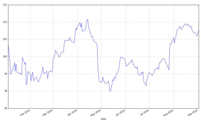
pandas_candlestick_ohlc(apple)   

燭狀圖中黑色線條代表該交易日閉市價格高于開市價格(盈利)，紅色線條代表該交易日開市價格高于閉市價格(虧損)。刻度線代表當天交易的最高價和最低價(影線用來指明燭身的哪端是開市，哪端是閉市)。燭狀圖在金融和技術分析中被廣泛使用在交易決策上，利用燭身的形狀，顏色和位置。我今天不會涉及到策略。

我們也許想要把不同的金融商品呈現在一張圖上：這樣我們可以比較不同的股票，比較股票跟市場的關系，或者可以看其他證券，例如交易所交易基金(ETFs)。在后面的內容中，我們將會學到如何畫金融證券跟一些指數(移動平均)的關系。屆時你需要使用線段圖而不是燭狀圖。(試想你如何重疊不同的燭狀圖而讓圖表保持整潔?)

下面我展示了不同技術公司股票的數據，以及如何調整數據讓數據線聚在一起。

microsoft = web.DataReader("MSFT", "yahoo", start, end) 
 
google = web.DataReader("GOOG", "yahoo", start, end) 
 
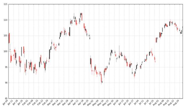
# Below I create a DataFrame consisting of the adjusted closing price of these stocks, first by making a list of these objects and using the join method 
 
stocks = pd.DataFrame({"AAPL": apple["Adj Close"], 
 
                      "MSFT": microsoft["Adj Close"], 
 
                      "GOOG": google["Adj Close"]}) 
 
stocks.head() 

stocks.plot(grid = True) 

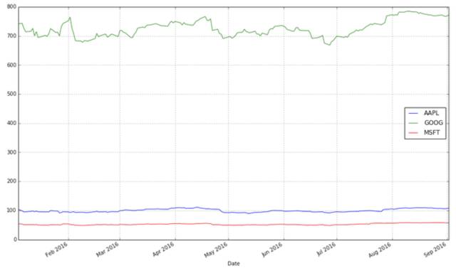
這張圖表的問題在哪里呢?雖然價格的絕對值很重要(昂貴的股票很難購得，這不僅會影響它們的波動性，也會影響你交易它們的難易度)，但是在交易中，我們更關注每支股票價格的變化而不是它的價格。Google的股票價格比蘋果微軟的都高，這個差別讓蘋果和微軟的股票顯得波動性很低，而事實并不是那樣。

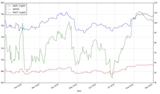
一個解決辦法就是用兩個不同的標度來作圖。一個標度用于蘋果和微軟的數據;另一個標度用來表示Google的數據。

stocks.plot(secondary_y = ["AAPL", "MSFT"], grid = True) 

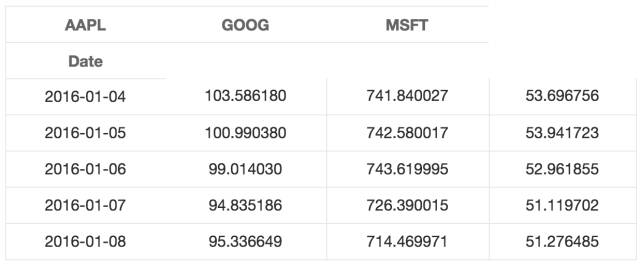
一個“更好”的解決方法是可視化我們實際關心的信息：股票的收益。這需要我們進行必要的數據轉化。數據轉化的方法很多。其中一個轉化方法是將每個交易日的股票交個跟比較我們所關心的時間段開始的股票價格相比較。也就是：

這需要轉化stock對象中的數據，操作如下：

# df.apply(arg) will apply the function arg to each column in df, and return a DataFrame with the result 
 
# Recall that lambda x is an anonymous function accepting parameter x; in this case, x will be a pandas Series object 
 
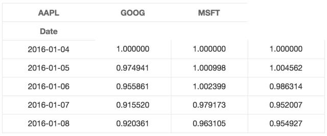
stock_return = stocks.apply(lambda x: x / x[0]) 
 
stock_return.head()  

stock_return.plot(grid = True).axhline(y = 1, color = "black", lw = 2)  

[[195993]] 

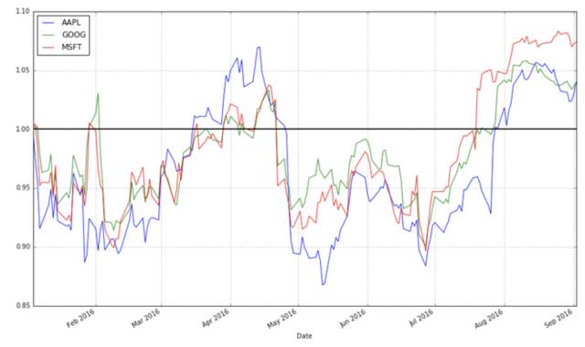
這個圖就有用多了。現在我們可以看到從我們所關心的日期算起，每支股票的收益有多高。而且我們可以看到這些股票之間的相關性很高。它們基本上朝同一個方向移動，在其他類型的圖表中很難觀察到這一現象。

我們還可以用每天的股值變化作圖。一個可行的方法是我們使用后一天$t + 1$和當天$t$的股值變化占當天股價的比例： 

我們也可以比較當天跟前一天的價格：

以上的公式并不相同，可能會讓我們得到不同的結論，但是我們可以使用對數差異來表示股票價格變化：

(這里的 

是自然對數,我們的定義不完全取決于使用 

 還是 

.) 使用對數差異的好處是該差異值可以被解釋為股票的百分比差異，但是不受分母的影響。

下面的代碼演示了如何計算和可視化股票的對數差異：

# Let's use NumPy's log function, though math's log function would work just as well 
 
import numpy as np 
 
stock_change = stocks.apply(lambda x: np.log(x) - np.log(x.shift(1))) # shift moves dates back by 1. 
 
stock_change.head() 

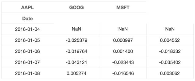
stock_change.plot(grid = True).axhline(y = 0, color = "black", lw = 2)  

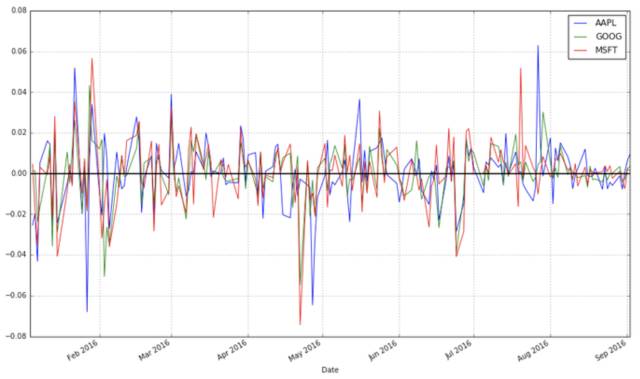
你更傾向于哪種轉換方法呢?從相對時間段開始日的收益差距可以明顯看出不同證券的總體走勢。不同交易日之間的差距被用于更多預測股市行情的方法中，它們是不容被忽視的。

移動平均值

圖表非常有用。在現實生活中，有些交易人在做決策的時候幾乎完全基于圖表(這些人是“技術人員”，從圖表中找到規律并制定交易策略被稱作技術分析，它是交易的基本教義之一。)下面讓我們來看看如何找到股票價格的變化趨勢。

一個q天的移動平均值(用 

來表示)定義為：對于某一個時間點t，它之前q天的平均值。

移動平均值可以讓一個系列的數據變得更平滑，有助于我們找到趨勢。q值越大，移動平均對短期的波動越不敏感。移動平均的基本目的就是從噪音中識別趨勢。快速的移動平均有偏小的q，它們更接近股票價格;而慢速的移動平均有較大的q值，這使得它們對波動不敏感從而更加穩定。

pandas提供了計算移動平均的函數。下面我將演示使用這個函數來計算蘋果公司股票價格的20天(一個月)移動平均值，并將它跟股票價格畫在一起。

apple["20d"] = np.round(apple["Close"].rolling(window = 20, center = False).mean(), 2) 
 
pandas_candlestick_ohlc(apple.loc['2016-01-04':'2016-08-07',:], otherseries = "20d") 

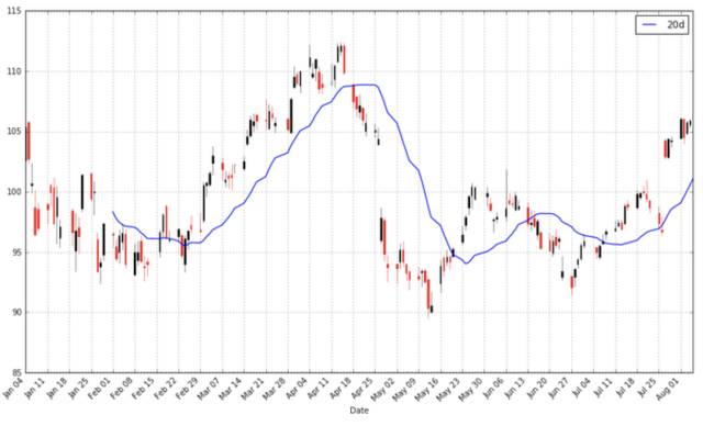
注意到平均值的起始點時間是很遲的。我們必須等到20天之后才能開始計算該值。這個問題對于更長時間段的移動平均來說是個更加嚴重的問題。因為我希望我可以計算200天的移動平均，我將擴展我們所得到的蘋果公司股票的數據，但我們主要還是只關注2016。

start = datetime.datetime(2010,1,1) 
 
apple = web.DataReader("AAPL", "yahoo", start, end) 
 
apple["20d"] = np.round(apple["Close"].rolling(window = 20, center = False).mean(), 2) 
 
pandas_candlestick_ohlc(apple.loc['2016-01-04':'2016-08-07',:], otherseries = "20d") 

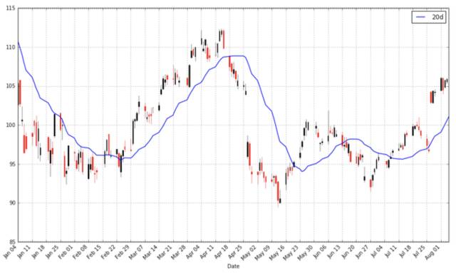
你會發現移動平均比真實的股票價格數據平滑很多。而且這個指數是非常難改變的：一支股票的價格需要變到平局值之上或之下才能改變移動平均線的方向。因此平均線的交叉點代表了潛在的趨勢變化，需要加以注意。

交易者往往對不同的移動平均感興趣，例如20天，50天和200天。要同時生成多條移動平均線也不難： 

apple["50d"] = np.round(apple["Close"].rolling(window = 50, center = False).mean(), 2) 
 
apple["200d"] = np.round(apple["Close"].rolling(window = 200, center = False).mean(), 2) 
 
pandas_candlestick_ohlc(apple.loc['2016-01-04':'2016-08-07',:], otherseries = ["20d", "50d", "200d"]) 

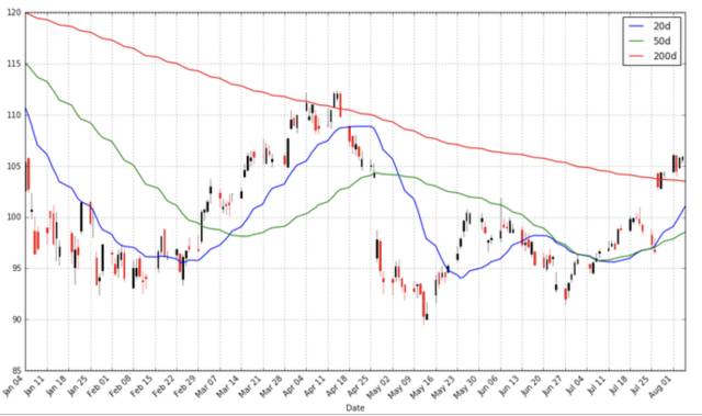
20天的移動平均線對小的變化非常敏感，而200天的移動平均線波動最小。這里的200天平均線顯示出來總體的熊市趨勢：股值總體來說一直在下降。20天移動平均線所代表的信息是熊市牛市交替，接下來有可能是牛市。這些平均線的交叉點就是交易信息點，它們代表股票價格的趨勢會有所改變因而你需要作出能盈利的相應決策。

更新：該文章早期版本提到算法交易跟高頻交易是一個意思。但是網友評論指出這并不一定：算法可以用來進行交易但不一定就是高頻。高頻交易是算法交易中間很大的一部分，但是兩者不等價。